Simulated Electrochemistry, part 4: Anodic Stripping Voltammetry
[chemistry mathematica montecarlo science teaching electrochem chiguiro We continue our series on Monte Carlo simulations of electrochemical processes with a treatment of anodic stripping voltammetry…
Motivating Experiment
Researchers have used chiguiro hair and poop to monitor environmental heavy metal contamination in Brazil. While these studies used ICP-OES to quantify the metal concentration, anodic stripping voltammetry (ASV) is an alternative electrochemical method used to measure heavy metals. An ASV experiment has two parts: First, the metal is accumulated at the working electrode by running at a constant reducing potential; this accumulation process improves the detection limit. Second, the metal is stripped from the surface by electrochemical oxidation; the current peak is used to quantify the concentration. According to IUPAC: “A peak-shaped anodic stripping voltammogram is obtained. Peak current depends on time of accumulation, mass transport of analyte (stirring), scan rate and mode (linear or pulse), and analyte concentration in solution.” Borrill et al. (2019) provide a tutorial review of ASV for heavy metal detection.
This should give us a few variables to study by Monte Carlo simulation. ROCK ON!
ImageSynthesize["A capybara playing in a 1980s heavy metal band"]

(aside: the last time I was in Berlin, I enjoyed an exhibit on Heavy Metal in East Germany #HeavyMetalinderDDR )
Defining the Voltage Program
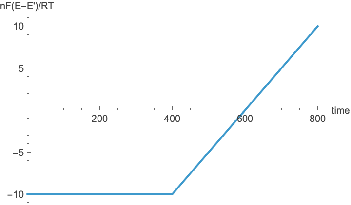
Define a function to make a simple linear ASV program, look at an example:
asvLinear[vStart_, vEnd_, tAccumulate_Integer, tRamp_Integer] := With[
    {accumulate = ConstantArray[vStart, tAccumulate],
     ramp = Rest@Subdivide[vStart, vEnd, tRamp]},
    Join[accumulate, ramp]]

expt = asvLinear[-10., 10., 400, 400];
ListLinePlot[expt, AxesLabel -> {"time", "nF(E-E')/RT"}]
Monte Carlo Simulation
Following closely on the approach introduced in Part 1, we simulate the one-dimensional diffusion problem using a discrete-time-step Monte Carlo simulation. The analyte begins in the oxidized state (M+) in solution at some random position in solution, and then takes a random walk during its trajectory. If it reaches the electrode, then it has the possibility of reacting as governed by the Boltzmann-Nernst probability. The primary difference here is that if the molecule is reduced, it is deposited on the surface (i.e., it remains at x = 0), corresponding to the reaction M+ + e- -> M(surface). Therefore, we must modify the reaction process so that it includes the position change move. The minor modifications are indicated with comments:
asvF = FunctionCompile@Function[
    {Typed[vv, TypeSpecifier["PackedArray"]["Real64", 1]],
     Typed[maxX, TypeSpecifier["Integer16"]]},
    Module[
     {x =  RandomInteger[{1, maxX}],
      state = +1,                                             (*!! start in oxidized state in solution *)
      obs = ConstantArray[0, Length[vv]],
      dx = 2 RandomInteger[{0, +1}, Length[vv]] - 1},
     Do[
      If[state == +1, x += dx[[t]];];                         (*!! only oxidized metal is mobile *)
       If[x == 0,
        If[RandomReal[] < 1./(1. + Exp[-vv[[t]]]),
          If[state == -1, (obs[[t]] = +1; state = +1; x = 1;), x = 1;], (*!! M-->M+ and moves back to soln, or unreacted M+ returns to soln *)
          If[state == +1, (obs[[t]] = -1; state = -1; x = 0;), x = 0;]  (*!! M+->M and added to surface, or unreacted M remains on surface *)
         ];
       ];
      , {t, Length[vv]}];
     obs
    ]]

All of the previously discussed caveats apply: This model omits convection, migration, double-layer current, surface saturation, competing reactions, and re-deposition after stripping. Additionally, the stripping-potential distribution is an ideal reversible thermodynamic model rather than a detailed treatment of nucleation, alloy formation, heterogeneous kinetics, or diffusion and re-deposition of stripped ions. Nevertheless, our premise is that this simplified model suffices to describe the key aspects of preconcentration and release phenomena observed in an ASV experiment.
Notional Experiment
Before exploring the different variables, let us take a quick look at what the expected current response will be over the course of such an experiment. Run a simple simulation with a 400-time-step accumulation stage followed by a 400-time-step stripping stage, and plot the result:
expt =  asvLinear[-10., 10., 400, 400];
obs = ParallelSum[asvF[expt, Ceiling[6*Sqrt[0.5*800]]], {i, 10^7}];
ListPlot[obs, AxesLabel -> {"time", "current"}, PlotRange -> All]
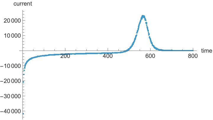
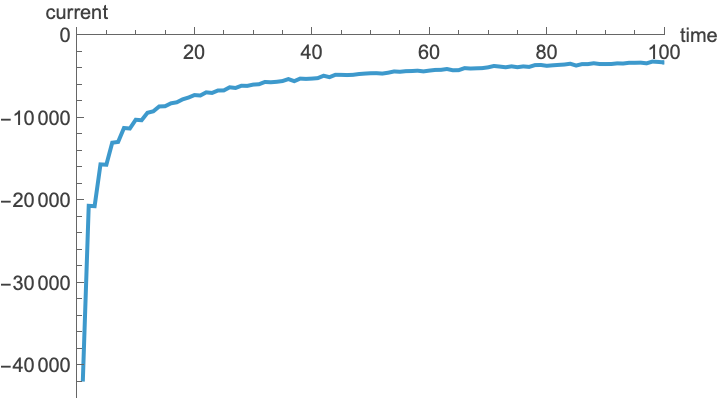
Let us take a closer look at the early time period. The negative deposition current is largest initially and decays as nearby ions are consumed. Its cumulative magnitude is the surface inventory available for stripping:
ListLinePlot[obs, AxesLabel -> {"time", "current"}, PlotRange -> { {0, 100}, {All, 0}}]
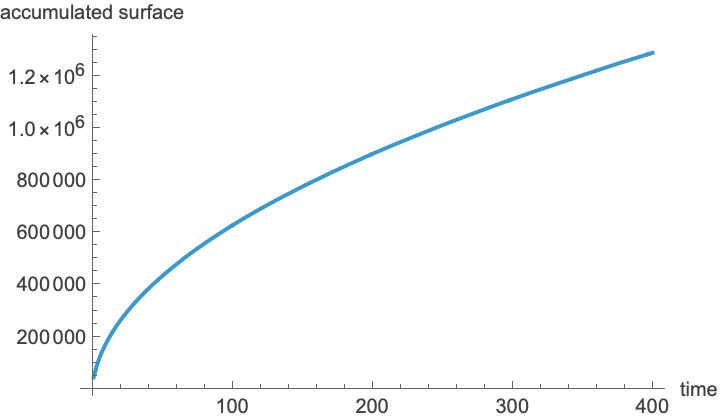
The cumulative magnitude is the surface inventory available for stripping:
ListLinePlot[Accumulate[-obs[[;; 400]]], AxesLabel -> {"time", "accumulated surface"}]
-Total@obs[[;; 400]] (* total # of species reduced to surface*)
(*1286046*)
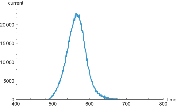
During the desorption step, we get a sharp spike as the metal gets oxidized off the surface:
ListLinePlot[obs, AxesLabel -> {"time", "current"}, PlotRange -> { {400, 800}, {0, All}}]
Total@obs[[401 ;;]] (* total # of species reduced to surface*)
(*1286042*)
Overall, nearly all of the deposited material gets released again (negative numbers indicate additional atoms remaining on the surface because the reduction-stage current has a negative sign):
Total[obs]

(*-4*)
Peak Current Depends on Time of Accumulation
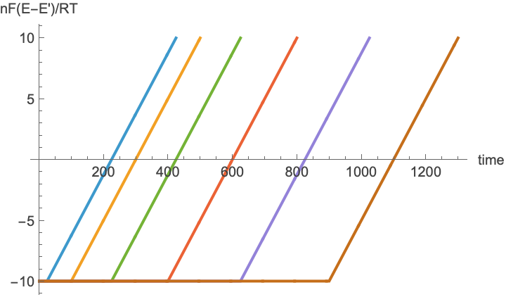
According to IUPAC: “Peak current depends on time of accumulation, mass transport of analyte (stirring), scan rate and mode (linear or pulse), and analyte concentration in solution.” So let us begin with the first of these. Define a series of experiments where we explore a range of different accumulation times; without malice aforethought, we will sample different values of the square root of the accumulation time:
accumulationTimes = Table[sqrtt^2, {sqrtt, 5, 30, 5}];
accumulationExpts = Table[ asvLinear[-10., 10., t, 400], {t, accumulationTimes}];
ListLinePlot[%, AxesLabel -> {"time", "nF(E-E')/RT"}]
Determine the maximum distance over which to sample for all of the simulations based on the last (longest) experiment, and then run the simulations. You can use fewer samples (e.g., 10^6) to run it faster, but the data will be noisier. You can also try using RemoteBatchMapSubmit, as demonstrated in the Part 3 tutorial, but we shall just run it locally for simplicity:
maxConc = With[
     {maxTime = Length@Last@accumulationExpts},
     Ceiling[6*Sqrt[0.5*maxTime]]];

accumulationObs = ParallelSum[asvF[#, maxConc], {i, 10^7}] & /@ accumulationExpts;
Extract the peak heights (with Gaussian smoothing over 10 time steps) during the stripping stage, perform a linear fit, and plot the results:
accumulationData = Transpose[
    {Sqrt[accumulationTimes], (Last@First@FindPeaks[#, 10]) & /@ accumulationObs[[All, -400 ;;]]}];
accumulationModel = ModelFit[accumulationData, "Linear"]

Show[
  ListPlot[
   List /@ accumulationData,
   PlotMarkers -> {"\[FilledCircle]", Medium},
   Frame -> True, FrameLabel -> {"Square root of Accumulation time", "Peak current"}],
  Plot[accumulationModel[x], {x, 0, Max[accumulationTimes]}, PlotStyle -> LightGray]]

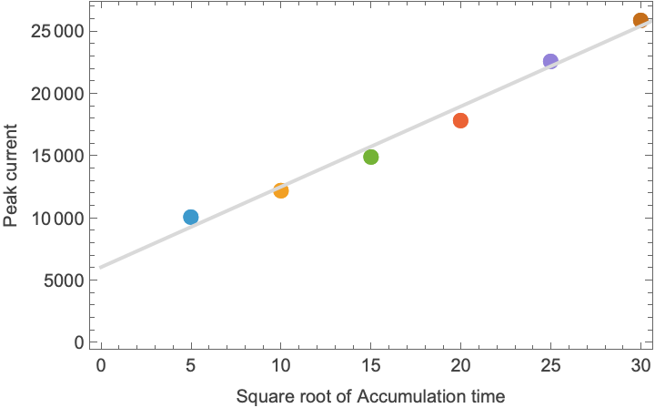
Conclusion: Qualitatively, one expects the peak current to increase with increasing accumulation time because, intuitively, we are giving more particles a chance to diffuse to the surface, and thus we accumulate more reduced metal on the surface to later oxidize during the stripping stage. Because our simulation has no stirring, this is diffusion-limited, and thus has a square-root dependence on the accumulation time. In a typical lab experiment, one would likely stir the vessel, in which case a linear dependence might be observed, provided that the analyte has not been depleted.
Peak Current Depends on Scan Rate
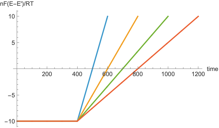
Continuing through the IUPAC statement: “Peak current depends on … scan rate…” Define a series of experiments where we explore different stripping times; the scan rate is inversely proportional to this scan time:
scanTime = Table[t, {t, 200, 800, 200}];
scanRateExpts = Table[ asvLinear[-10., 10., 400, t], {t, scanTime}];
ListLinePlot[%, AxesLabel -> {"time", "nF(E-E')/RT"}]
As before, define an appropriate maximum distance to avoid diffusion limiting our simulation, and run the simulation:
maxConc = With[
     {maxTime = Length@Last@scanRateExpts},
     Ceiling[6*Sqrt[0.5*maxTime]]];

scanRateObs = ParallelSum[asvF[#, maxConc], {i, 10^7}] & /@ scanRateExpts;
Intuitively, the stripping step removes a more or less fixed quantity of accumulated material from the electrode, so increasing the scan rate (i.e., using a short scan time) compresses that charge into a shorter interval of time, thus increasing the current. Indeed, we see a taller, sharper peak as the scan rate increases:
ListLinePlot[
  scanRateObs,
  AxesLabel -> {"time", "current"},
  PlotLegends -> Placed[scanTime, {Right, Top}],
  PlotRange -> { {400, 900}, {0, All}}]
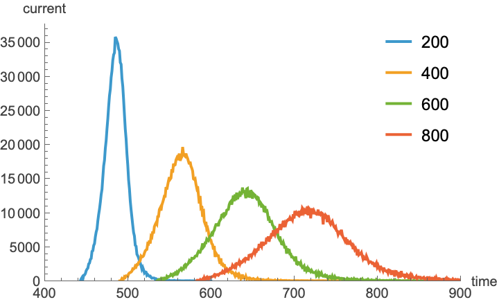
We can confirm our intuition that the amount of adsorbed material accumulated on the electrode is approximately constant by checking whether the integrated stripping current (i.e., total number of electrons = total number of desorbed metal atoms) is about the same for all cases:
Total /@ scanRateObs[[All, 400 ;; UpTo[900]]]

(*{1048520, 1048418, 1050155, 1043866}*)
In each case, the stripping is nearly complete:
Total /@ scanRateObs

(*{-2, -4, -1, -1}*)
Finally, determine the quantitative relationship between the stripping scan rate and observed peak current:
scanRateData = Transpose[
   {20./scanTime,
    (Last@First@FindPeaks[#, 10]) & /@ scanRateObs[[All, 400 ;; UpTo[900]]]}]
scanRateModel = ModelFit[scanRateData, "Linear"]

Show[
  ListPlot[
   List /@ scanRateData,
   PlotMarkers -> {"\[FilledCircle]", Medium},
   Frame -> True, FrameLabel -> {"Scan rate (dV/dt)", "Peak current"}],
  Plot[scanRateModel[x], {x, 0, 0.2}, PlotStyle -> LightGray]]

(*{ {0.1, 35781}, {0.05, 19639}, {0.0333333, 13688}, {0.025, 10933}}*)

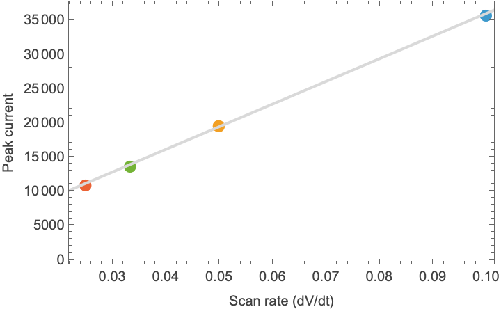
Conclusion: We confirm the expected linear relationship between the stripping scan rate and observed peak current. It is also interesting to compare this to the behavior of the Randles–Ševčík equation studied in an earlier post. You will recall that the Randles–Ševčík equation predicts a square-root dependence on the scan rate resulting from diffusion processes, in contrast to the linear behavior observed here which results from surface-confined processes. In the lab, this might be used for mechanistic determination.
Peak Current Depends on Analyte Concentration
Onward! IUPAC also told us: “Peak current depends on … analyte concentration in solution.” We saw in Part 2 and Part 3 how to treat concentration changes by sampling the molecule positions over a longer interval of possible starting positions. To see the power of ASV, we will simulate a two-order-of-magnitude change in the concentration, using a fast stripping step to get a higher peak:
expt = asvLinear[-10., 10., 400, 200];
maxConc = Ceiling[6*Sqrt[0.5*Length[expt]]];
concentrations  = {1.0, 0.5, .1, 0.05, 0.01};
job = RemoteBatchMapSubmit[ (* ...or just use Map to run locally *)
   ParallelSum[asvF[expt, #], {i, 10^7}] &,
   Round[(maxConc/concentrations)]]

Inuitively, one expects the stripping current (as a function of time) to be proportional to the concentration, as at high concentration, more metal atoms will get added to the surface during the accumulation step:
concentrationObs = job["EvaluationResults"];
ListLinePlot[
  concentrationObs,
  AxesLabel -> {"time", "current"},
  PlotLegends -> Placed[concentrations, {Right, Top}],
  PlotRange -> { {425, 550}, {0, All}}]
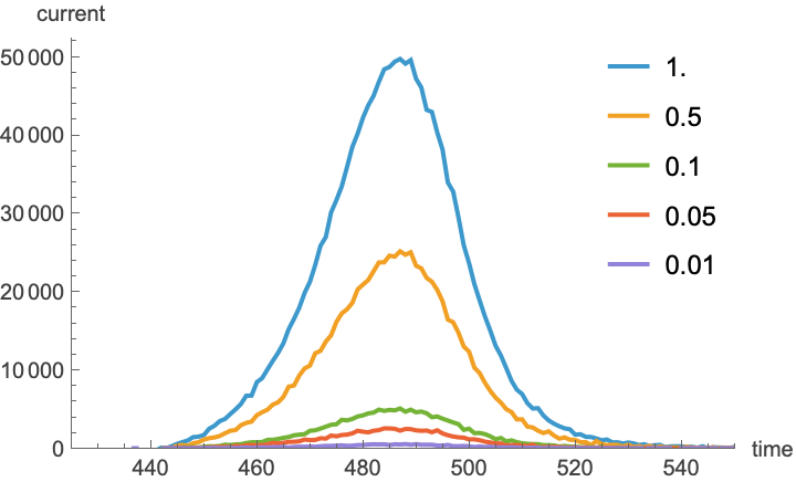
Indeed, we see a linear dependence on concentration over two orders of magnitude:
concentrationData = Transpose[{concentrations, (Last@First@FindPeaks[#, 10]) & /@ concentrationObs[[All, 450 ;; 550]]}];
concentrationModel = ModelFit[%, "Linear"]

Show[
  ListPlot[
   List /@ concentrationData,
   PlotMarkers -> {"\[FilledCircle]", Medium},
   Frame -> True, FrameLabel -> {"Concentration", "Peak current"}],
  Plot[concentrationModel[x], {x, 0, 1}, PlotStyle -> LightGray]]

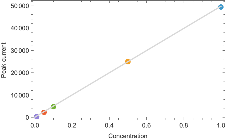
An astute reader might object: the fitted model does not have an intercept of zero (i.e., it predicts that there should be a small current even in the absence of analyte), and we might try this the old-fashioned way if you are a stickler for detail, but it does not really matter:
LinearModelFit[concentrationData, {x}, x, IncludeConstantBasis -> False]

Ideas for Future Work
We have simulated linear stripping voltammetry, but in practice this can result in the measured current having both the faradaic (from metal stripping) and non-faradaic (background currents such as capacitance) components. Consequently, square-wave voltammetry and other methods are adopted. See the Borrill et al. review for more details and Rodeostat blog for a demonstration experiment. The simulation could be modified to account for these different potential changes as a function of time, perhaps with some special handling of the accumulation data needed for differential-pulse voltammetry.
Another possible extension would be to generalize the code to allow for multiple analytes with different formal potentials and/or diffusion coefficients. Their deposited inventories would then generate separate stripping peaks, demonstrating simultaneous identification and quantification without changing the basic simulation architecture.
These are both left as an exercise for the reader.
Conclusions
Our simple Monte Carlo method, with small modifications, can adequately describe the effects of accumulation time, scan rate, and concentration on the observed peak current in an ASV experiment. This is simple enough for a chiguiro to understand and use in the laboratory. Because chiguiros do not have much spare brain power, avoiding lead helps keep them smart enough to do electrochemistry experiments.
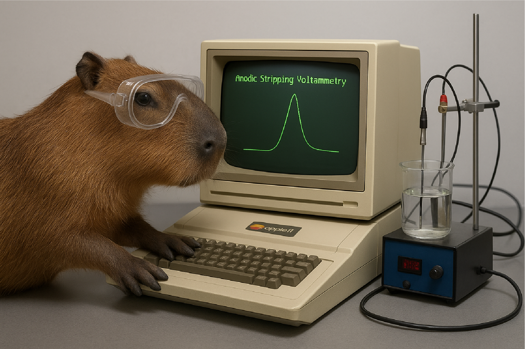
ImageSynthesize[
  "A photorealistic capybara wearing laboratory safety goggles typing on an Apple ][ computer which is connected to an experimental apparatus.  On the screen in green print is a figure related to anodic stripping voltammetry. The Voltammogram should only have a single peak (it is *not* a cyclic voltammetry)."]
ToJekyll["Simulated Electrochemistry, part 4: Anodic Stripping Voltammetry",
  "chemistry mathematica montecarlo science teaching electrochem chiguiro"]
Monte Carlo Simulations of Electrochemistry
- Part 1: Monte Carlo Simulation of Diffusion, Chronoamperometry, Linear & Cyclic Voltammetry
- Part 2: Reproducing the Randles–Ševčík Relation
- Part 3: Irreversible Cyclic Voltammetry and Quantification
- Part 4: Anodic Stripping Voltammetry — this post
- Part 5: Optimizing the Monte Carlo Simulation
- Part 6: Concentration Profiles During Cyclic Voltammetry