Simulated Electrochemistry

I spent some time this summer diving into electrochemistry, which included vibe coding some HTML5 and Mathematica potentiostat interfacing software, and reading Eliaz and Gileadi, Physical Electrochemistry: Fundamentals, Techniques, and Applications and Honeychurch, Simulating electrochemical reactions with Mathematica (but skip the book and use updated version posted by the author on github), the latter having been recommended to me many years ago by BobTheChemist. While I enjoyed the premise of Honeychurch’s book, in working through it myself, I found many opportunities to improve the presentation and simplicity of the code. Implementing improved and simplified Monte Carlo simulations of chronoamperometry, linear sweep voltammetry, and cyclic voltammetry helped me solidify my atomistic mental picture…

A longer comment on Honeychurch: Much of his book is spent on implementing differential equation integration algorithms, with time spent on building up both procedural and functional implementations of these algorithms while explaining the rationale. While interesting (and I have notes towards simplification/clarification of those as well), a notable omission is the use of the finite element capabilities which have been added to Mathematica since the original publication (I have some notes on that too…). The notes below are inspired by his Chapter 12 on Monte Carlo simulations, but very little of the code is the same. In general, implementing the Monte Carlo simulations helped me understand the underlying physical processes better (good!) but felt that Honeychurch introduced some unnecessary complications in handling the simulation outcomes that obscured that simple physical picture (at least for me). The notes below are the result of trying to make the code as simple (and fast!) as possible for beginners, as well as explore some features in the new Mathematica 15. Rather than unpack each function, I have tried to keep the functions short and assume the reader can dissect them as necessary. Although I generally prefer a functional style these days, the voltammetry simulation is dramatically simpler in procedural style, so I just stick with that. De gustibus non est disputandum.

Random Walks and Diffusion

(This type of content is in my Computational Models of Biochemistry course, so I have thought about teaching it to beginners before…)

Diffusion can be modelled as a random walk of molecules in a solution. Our general strategy will be to simulate the trajectory of an individual molecule as it takes random steps of +1 or -1. Let us begin with a one-dimensional simulation which allows us to specify an initial position, x0, and number of steps over which to evolve the particle:

rw[x0_Integer, nSteps_Integer] := x0 + Accumulate@RandomChoice[{-1, +1}, nSteps]

ListLinePlot[rw[0, 20], AxesLabel -> {"t", "x"}]

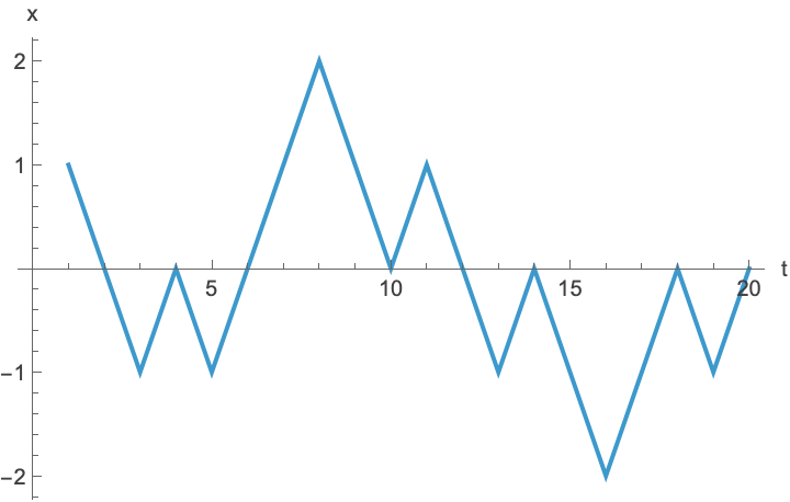
(Notice how we have generated all of the random numbers in a single batch; this is often faster than many separate single random number selections, at the cost of the memory needed to store those values.)

What is the distribution of final positions, after a particle released at x = 0 is allowed to evolve for 20 time steps? Evaluate this over a sample of 5000 trajectories:

time = 20;
number = 5000;
data = Table[ Last@rw[0, time], {number}];

Histogram[data, AxesLabel -> {"x", "count"}]

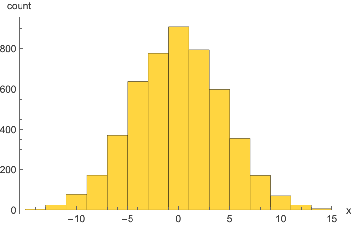
Observe the Gaussian-type distribution of final positions from our simulation. The theory of random walks tells us that the probability of the particle being a P, of a molecule being located at a distance, $x$, after time t (moving a distance $d$ per time increment τ) will have a Gaussian distribution given by: P(x,t) ≈ √(2τ/(πt)) exp(−x²τ/(2d²t)).

And the corresponding diffusion coefficient, D = d²/(2τ),

Therefore, our simulation (with t = 20, d = 1, τ = 1) mimics a system with D = 0.5 and analytic probability distribution

Sqrt[2./(Pi*time)]* Exp[-x^2/(2.*time)]

(*0.178412 \[ExponentialE]^(-0.025 x^2)*)

How well do the simulated results agree with the analytical form of the diffusion equation? First, generate a list of {final-position, proportion-of-outcomes-at-that-position} pairs:

m1 = List @@@ Normal@N@KeySort@ResourceFunction["Proportions"]@data

(*{ {-14, 0.0008}, {-12, 0.0052}, {-10, 0.0156}, {-8, 0.0346}, {-6, 0.0742}, {-4, 0.1278}, {-2, 0.1556}, {0, 0.1818}, {2, 0.159}, {4, 0.1196}, {6, 0.0712}, {8, 0.0344}, {10, 0.0142}, {12, 0.0048}, {14, 0.0012}}*)

Mathematica 15 introduced a new ModelFit function which simplifies various downstream tasks, such as plotting the fit atop data:

model = ModelFit[m1, FormulaModel[A Exp[-x^2/b], {A, b}, x]] (* new in v15 *)

Histogram[data, Automatic, "Probability", PlotFit -> model]

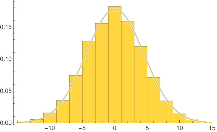
Consequently we see good agreement between the simulation and the exact result.

Random walks in higher dimensions

The same strategy can be generalized to two-dimensional and three-dimensional random walks in a straightforward way by representing the position and the changes as vectors:

rw2[x0_ : {0, 0}, nSteps_ : 2000] := (x0 + #) & /@ 
  Accumulate@RandomChoice[{ {1, 0}, {-1, 0}, {0, 1}, {0, -1}}, nSteps]

ListLinePlot[rw2[], AxesLabel -> {"x", "y"}] 

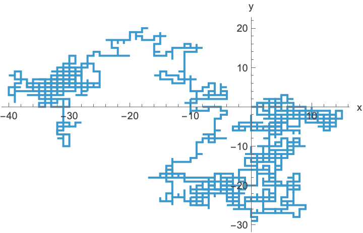
Rather than adding the initial position to each entry, it may be more natural to think about this as a nest-type function application, where we update the current position by a single random choice:

rw2[x0_ : {0, 0}, nSteps_ : 2000] := 
  NestList[# + RandomChoice[{ {1, 0}, {-1, 0}, {0, 1}, {0, -1}}] &, x0, nSteps]

It would still be possible to pre-generate the list of RandomChoices by using a fold-type operation instead:

rw2[x0_ : {0, 0}, nSteps_ : 2000] := 
  With[
   {dx = RandomChoice[{ {1, 0}, {-1, 0}, {0, 1}, {0, -1}}, nSteps]}, 
   FoldList[Plus, x0, dx]]

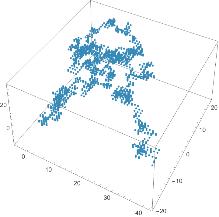
The same logic can be used to extend the result to three-dimensions:

rw3[x0_ : {0, 0, 0}, nSteps_ : 2000] := With[
    {step := RandomChoice[{ {1, 0, 0}, {-1, 0, 0}, {0, 1, 0}, {0, -1, 0}, {0, 0, 1}, {0, 0, -1}}]}, 
    NestList[# + step &, x0, nSteps]] 
 
ListPointPlot3D[rw3[], AspectRatio -> 1]

Chronoamperometric simulation

(Honeychurch leaves this to the end of the chapter, but as it is a much simpler application, I think it makes better pedagogical sense to introduce it before voltammetric simulations.)

In chronoamperometry, the electric potential of the working electrode is stepped from zero to a sufficiently high value to reduce any analyte that contacts it, and we measure the resulting current as a function of time. To simulate this, we assume that the molecules are uniformly randomly distributed in the solution. Before the working electrode is turned on, the molecule is at some random initial position x0, during the duration of the experiment (which we shall set to 400 time units), the molecule diffuses in 1D. If it contacts the electrode at x = 0, then it is reduced and the corresponding electron count is recorded. As the potential is sufficiently high, we may assume that the molecules are not re-oxidized, so we no longer need to consider that molecule. Our goal then is to determine the first timestep where x=0, as this is when a blip is contributed to the simulated current. As above we are going to write a function which simulates just a single molecule, and then aggregate those results. A reasonable first implementation is as follows:

timeToElectrode[x0_Integer, tMax_ : 400] := With[
   {randomWalk = x0 + Accumulate@RandomChoice[{-1, +1}, tMax]}, 
   LengthWhile[randomWalk, GreaterThan[0]]]

While this has a certain simplicity, it should be noted that the majority of molecule simulations run over all 400 timesteps without reacting, and so the outputs of 400 would need to be interpreted as no-reaction rather than reaction-at-400. (Additionally, there’s a subtle off-by-one counting error, as it reports the number of elements before zero is counted, rather than including it.) One can remove that complication and also achieve a 4.5x speedup by implementing the following (perhaps slightly more complicated) function instead:

timeToElectrode[x0_Integer, tMax_ : 400] := With[
   {randomWalk = x0 + Accumulate@RandomChoice[{-1, +1}, tMax]}, 
   First@FirstPosition[randomWalk, 0, Missing[Nothing]]]

(Logic: The third argument of FirstPosition gives an alternate response. First will take the first argument of the list or any other Head that is present, and thus it uncovers the Nothing inside the Missing head. Nothing entries in a list vanish when evaluated, avoiding the need to have a collection of non-events in the final list.)

Go ahead and run this over a sample of random starting positions:

ca = ParallelMap[
     timeToElectrode, 
     RandomInteger[{1, 85}, 10^6]]; // AbsoluteTiming

(*{5.29366, Null}*)

Interestingly, only 18% of our starting particles actually react:

Length[ca]/10^6 // N

(*0.181754*)

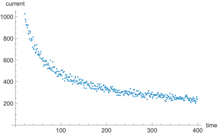
The output consists of the times when individual molecules reacted. The measured current (as a function of time) is the aggregated value of some number of events at each time during the experiment. So we want to make a list of {time, number-of-events} pairs:

ca2 = SortBy[First]@Tally[ca];
ListPlot[ca2, AxesLabel -> {"time", "current"}]

Aside: One might also consider BinCounts[ca,{1,400,1}], but only gives a list of {events-at-t1, events-at-t2, ...}. While that is fine for plotting, it makes the model fitting slightly more awkward.

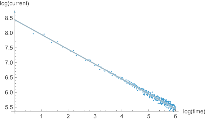
The Cottrell equation suggests that the slope of the log-log plot should be 1/2, and indeed this appears to be the case (it does not matter if you do this as the natural logarithm or log-base-10 (Log10), as this just changes the offset of the fit):

ModelFit[Log@ca2, "Linear"]
ListPlot[Log@ca2, PlotFit -> %, AxesLabel -> {"log(time)", "log(current)"}]

Linear sweep voltammetry

(The Honeychurch implementation involves some rather complicated data structure wrangling that, in my opinion, interferes with understanding the underlying simulation. In preliminary work, I explored some functional programming ways that mimic this, but they are considerably slower and more complicated. The below is a considerably simplified and fast approach. For comparison, Honeychurch mentions that his full simulation required 225 minutes; we shall do it in a fraction of a time, mostly on account of using a faster computer than his Macintosh 400 MHz G4 , but partly because of algorithmic improvements.)

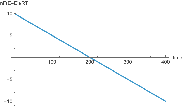
In linear sweep voltammetry one measures the current at the working electrode while the potential is changed linearly in time. For the sake of modeling, we set the zero to be the formal potential of our analyte species, and sweep from 10 nF/RT above to -10 nF/RT below that value over the 400 timestep experiment. Our potential sweep as a function of time looks like:

Clear[v, p, obs]
v0 = 10.;
incr = 0.05;
v = Table[v0 - t*incr, {t, 1, 400}]; (* or: N@Rest@Subdivide[v0,-v0,400] *)
ListPlot[v, AxesLabel -> {"time", "nF(E-E')/RT"}]

We implement the simulation by defining a function which takes as input the voltage as a function of time; the number of entries corresponds to the number of timesteps, i.e., the linear potential change is discretized to the timestep grid used in the simulation, and this is represented as a list of real numbers. The function should return an output vector, of the same length, of integers denoting oxidation or reduction events at each specific time. We avoid having to provide additional specifications of the simulation duration by using the Length of the input voltage list, and perform the sampling of initial molecule positions within the function itself. The simulation over the lifetime of a single molecule begins by sampling a possible initial position within the region, starting in the oxidized state. The obs list is used to store observed events, with each entry corresponding to a specific time (or voltage) of the experiment. By IUPAC convention, oxidation is represented with a positive current and reduction as a negative current. If the molecule reaches the electrode at x=0, then the Boltzmann probability, as determined from the applied potential, is used to compute the probability that the molecule should be reduced or oxidized. If the molecule is already in a state, no event occurs. A procedural implementation:

Clear[sweep]
sweep[v_List] := Module[
   {x = RandomInteger[{1, Ceiling[6*Sqrt[Length[v]/2]]}], (* sample within 6 Sqrt[D t] *)
    state = +1,                                           (* start in oxidized state *)
    obs = ConstantArray[0, Length[v]],                    (* store observed redox events *)
    dx = RandomChoice[{-1, +1}, Length[v]],               (* precompute steps *)
    xi}, 
   Do[
    x += dx[[t]];                                         (* update the particle position *)
     If[x == 0,                                           (* has particle hit the electrode? *)
      xi = Exp[v[[t]]];                                     (* compute Boltzmann factor for potential *)
      If[RandomReal[] < xi/(1. + xi),                       (* Does eqm favor oxidation or reduction? *) 
       If[state == -1, obs[[t]] = +1; state = +1;],           (* gets or remains oxidized*)
       If[state == +1, obs[[t]] = -1; state = -1;]            (* gets or remains reduced *) 
      ]; 
      x = 1; (* reset particle position *) 
     ]; 
    , {t, Length[v]}]; (* iterate over all times *)
   obs (* return the final observation vector *) 
  ]

As before, the observed current is the sum over a collection of these individual molecular events; computing this over a million molecules takes a minute or so:

AbsoluteTiming[
  obs = ParallelSum[sweep[v], {i, 10^6}];]

(*{86.7109, Null}*)

ListPlot[
  Transpose[{v, obs}], 
  Frame -> True, FrameLabel -> {"nF(E-E')/RT", "Current"}]

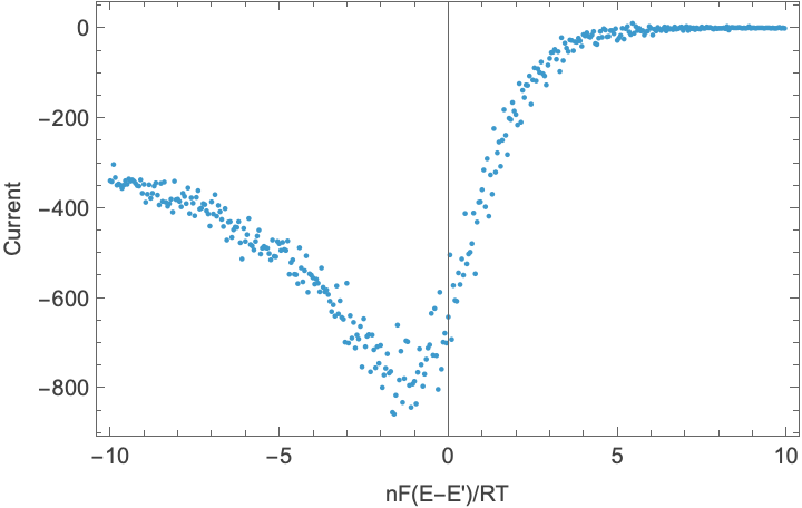
Our simulation captures the shape observed in the measured I-V curve of a reversible reaction; recall that we started the experiment with potential = +10, so read this from right to left. Initially, no current is observed because the potential is insufficiently negative to reduce the oxidized species and everything is already oxidized at the beginning of the simulation anyway. As the voltage is lowered, the surface concentration ratio between oxidized and reduced species is driven by the Nernst equation relationship, resulting in reduction of the molecules (negative current). A local minimum results because of the diffusion limit of getting new oxidized molecules to the electrode.

The result is noisy, as only a few hundred events are observed at any particular value of the potential, and the only straightforward path for improving that is to run more trajectories (with the signal-to-noise ratio scaling with the square-root of examples) or else to try some fitting/smoothing to the results.

Compilation for Speed

The simulation can be accelerated by compiling the function; this requires some small modification, mainly around variable type handling. (Mathematica has two paths for compilation, Compile and FunctionCompile; we shall use the latter, which is a newer (introduced in v.12), more restrictive, but potentially faster method, for the sake of illustrating type related issues):

Clear[vv]; 
 
sweepF = FunctionCompile@Function[ (* compile a pure function definition *)
    Typed[vv, TypeSpecifier["PackedArray"]["Real64", 1]], (* !! explicit input data type *)
    Module[
     {x =  RandomInteger[{1, Ceiling[6.*Sqrt[0.5*Length[vv]]]}], (*!! force real arg to Sqrt *)
      state = +1, 
      obs = ConstantArray[0, Length[vv]], 
      dx = 2 RandomInteger[{0, +1}, Length[vv]] - 1, (* !! precompute steps, guaranteed integer *)
      xi}, 
     Do[
      x += dx[[t]]; 
       If[x == 0, 
        xi = Exp[vv[[t]]]; 
        If[RandomReal[] < xi/(1. + xi), 
         If[state == -1, obs[[t]] = +1; state = +1;], 
         If[state == +1, obs[[t]] = -1; state = -1;] 
        ]; 
        x = 1; 
       ]; 
      , {t, Length[vv]}]; 
     obs 
    ]]

Comments indicate some special modifications required to avoid compilation errors. In addition to providing an explicit type specification for the input argument, some of the arithmetic and random number functions do not play well with the compiler. Specifically: Sqrt wants to have an explicitly real input argument, so use multiplication by 0.5 instead of divide by 2 to cast the result to real. RandomChoice does not provide a sufficient type guarantee for compilation, so use RandomInteger instead to achieve the same goal. Otherwise, very little changes, and the resulting compiled function can be used as before, but with a 10x speedup:

AbsoluteTiming[
  obs = ParallelSum[sweepF[v], {i, 10^6}];]

(*{9.41406, Null}*)

ListPlot[
  Transpose[{v, obs}], 
  Frame -> True, FrameLabel -> {"nF(E-E')/RT", "Current"}]

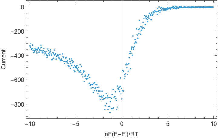
Running 10x faster means that we can run more trajectories for the same total computation time, which would allow us to improve the signal-to-noise ratio by about 3x (= Sqrt[10]) for a fixed computational budget of our original interpreted code.

To go even faster, the brute force way is just to parallelize over more cores (I only have 8 on my laptop) locally or to use a RemoteBatch job (although the initialization time is non-trivial). The smarter way would be to simulate multiple particle events inside the sweepF function so that it accumulates multiple trials in the same obs (saving a lot of arithmetic and memory), but this would move away from our initial design strategy of having each function simulate a single particle. If you pursue this, be sure to do something like obs[[t]]++ (instead of obs[[t]]=+1) to account for the fact that multiple events are being accumulated.

Optimization without compilation by skipping non-events

Our simulation is instructive, but quite inefficient. As we saw in the chronoamperometric simulation, only 18% of the particles reach the electrode. Similar statistics are observed in this simulation:

pContributing = (1. - #/10^5)&@
  Total@ParallelTable[Boole@ContainsOnly[{0}]@sweepF[v], {i, 10^5}]

(*0.135*)

This suggests that the minority of our simulations contributes to the final result. In most cases, either the particle never reaches the electrode or it fails to react for some reason. The former is likely to be dominant, based on the analysis of the chronoamperometry simulations. This suggests a modification to the non-compiled code where we check if the particle will ever hit the electrode; if not, then just Return the zero results immediately and skip the Do loop. While this wastes arithmetic operations, vectorized operations in the Mathematica interpreter are much faster than the overhead of explicit loops, and this allows us to achieve a 2.5x speedup over the previous interpreted version of the function:

Clear[sweep]
sweep[v_List] := Module[
    {x = RandomInteger[{1, Ceiling[6*Sqrt[Length[v]/2]]}], 
     state = +1, 
     obs = ConstantArray[0, Length[v]], 
     dx = RandomChoice[{-1, +1}, Length[v]], 
     xi}, 
    If[ContainsNone[x + Accumulate[dx], {0}], Return[obs]]; (* !! check possible x=0 states *)
    Do[
     x += dx[[t]]; 
      If[x == 0, 
       xi = Exp[v[[t]]]; 
       If[RandomReal[] < xi/(1. + xi), 
        If[state == -1, obs[[t]] = +1; state = +1;], 
        If[state == +1, obs[[t]] = -1; state = -1;] 
       ]; 
       x = 1; 
      ]; 
     , {t, Length[v]}]; 
    obs 
   ] 
 
AbsoluteTiming[
  obs = ParallelSum[sweep[v], {i, 10^6}];]

(*{31.0911, Null}*)

In principle, If[ContainsAny[x+Accumulate[dx],{0}], Null, Return[obs]]; is slightly faster because it can stop sooner, but for only 400 elements this does not make a noticeable difference.

However, including this precheck slows down the compiled function by 1.5-2 seconds, because of the additional arithmetic operations that are imposed. The take-home lesson here is that interpreted code can sometimes benefit from using vectorized operations to avoid a procedural loop. Indeed, 30 seconds for the simulation might be fast enough for exploratory purposes, limiting the motivation to pursue function compilation.

Cyclic Voltammetry

(Honeychurch could not treat this because of the slow simulations available; the faster simulation makes this a trivial extension.)

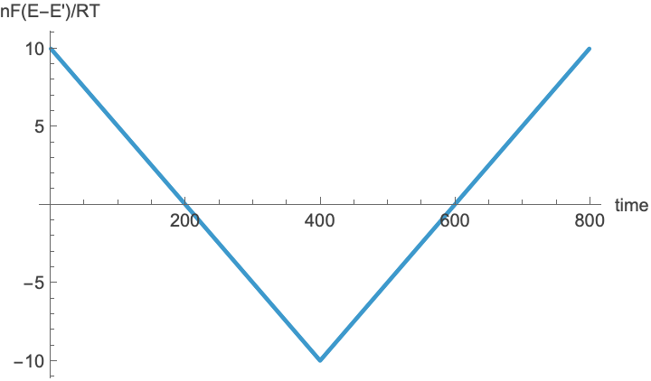
Cyclic voltammetry is a voltametric method where the potential is ramped linearly in time in a cyclic fashion. (See also the now-classic J Chem Educ 2017). No modification to the code is needed, we need only provide a revised list of voltages as a function of time:

cv = Join[v, Rest@Reverse[v]];
ListPlot[cv, AxesLabel -> {"time", "nF(E-E')/RT"}]

Surprisingly, the simulation takes very little additional time compared to the 400-timestep linear ramp, which suggests that the computational bottleneck is in parallelization setup, function initialization, and summing the results, rather than the internals of the simulation:

AbsoluteTiming[
  cvObs = ParallelSum[sweepF[cv], {i, 10^6}];]

(*{9.51525, Null}*)

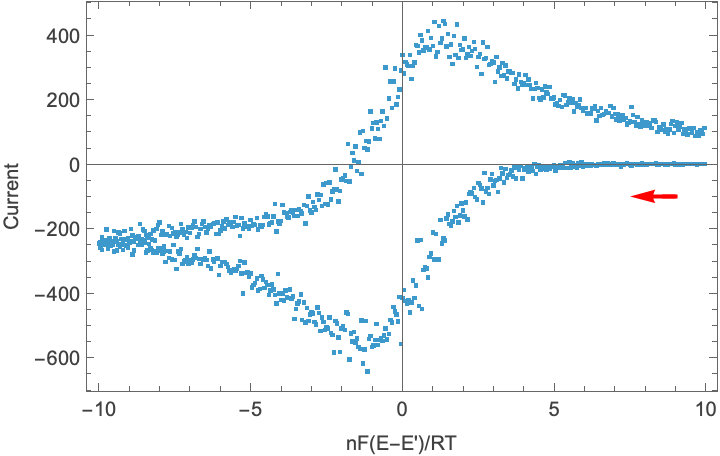
Here are the results plotted in the standard IUPAC convention (and thus may look weird to readers more familiar with the US convention, which rotates this by 180°):

ListPlot[
  Transpose[{cv, cvObs}], 
  Frame -> True, FrameLabel -> {"nF(E-E')/RT", "Current"}, 
  Epilog -> {Red, Thick, Arrow[{ {9, -100}, {7.5, -100}}]}]

Gratuitous GenAI content

Now that we’ve generated our cyclic voltagram: Quack quack! (As an aside, the voltammogram in the generated cartoon appears to follow the US convention rather than the IUPAC convention, illustrating the US-bias of frontier AI models.)

ImageSynthesize["Generate a cyclic voltammetry duck"]

However: it appears chiguiros are superior because they use the IUPAC standard convention by default…although they appear to have difficulty connecting the electrodes properly…

ImageSynthesize["Generate a cyclic voltammetry capybara"]

ToJekyll["Simulated Electrochemistry", "chemistry mathematica montecarlo science teaching"]

Monte Carlo Simulations of Electrochemistry

• Part 1: Monte Carlo Simulation of Diffusion, Chronoamperometry, Linear & Cyclic Voltammetry — this post
• Part 2: Reproducing the Randles–Ševčík Relation
• Part 3: Irreversible Cyclic Voltammetry and Quantification