Simulated Electrochemistry, part 2: The Randles-Ševčík Equation
[chemistry mathematica montecarlo science teaching electrochem chiguiro In our previous episode, we implemented a Monte Carlo simulation of chronoamperometry, linear sweep voltammetry, and cyclic voltammetry. In this episode, we adapt this to study the current dependence on scan rate and reproduce the Randles-Ševčík equation…
Setting the Scan rate
Experimentally, one varies the scanning rate and looks for changes in the peak current; faster scan rates lead to larger currents. To simulate this, as before, we define a list of the thermodynamically rescaled voltages relative to the redox potential of our molecule. Faster scan rates mean cycling the voltage from the maximum to minimum in fewer time steps. For convenience, define a helper function for the task:
Clear[cv]
cv[v0_, time_Integer] := With[
   {v = N@ Rest@ Subdivide[v0, -v0, time/2] },
   Join[v, Rest@ Reverse[v]]]
…and then use it to define several different one-pass cyclic voltammetry experiments:
expts = cv[10., #]& /@ {60, 120, 200, 250, 400};
ListLinePlot[%, AxesLabel -> {"time", "nF(E-E')/RT"}]
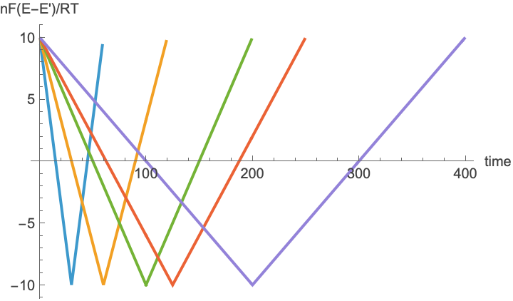
…having different scan rates:
rates = (#[[-1]] - #[[-2]])& /@ expts

(*{0.666667, 0.333333, 0.2, 0.16, 0.1}*)
Simulation function, revisited
You might be tempted to just throw these voltage functions into the previous simulation code, but this will introduce a subtle error. As you will recall, we sampled possible initial conditions of the molecule up to Ceiling[6 Sqrt[d t]], away from the electrode, where d = 0.5 is the diffusion coefficient and t is the maximum simulation time. This was done for the sake of computational efficiency–if time is short, the particle is unlikely to diffuse a long distance, and so sampling from far away would mean that even more events would result in no measurement. But if we naively do this and then try to compare experiments with different time durations, then each of the simulations will be sampling its (fixed) 10^6 trials over different volumes—effectively changing the concentration of our system. We can avoid this problem by modifying the function to take a fixed distance as input and using that for all simulations; when we run it, we shall provide the largest relevant value. (Alternatively, we could also run different numbers of trials, but that would be more complicated.) The code below marks changes with comments:
sweepF = FunctionCompile@Function[
    {Typed[vv, TypeSpecifier["PackedArray"]["Real64", 1]],
     Typed[maxX, TypeSpecifier["Integer16"]]},     (* !! define fixed length *)
    Module[
     {x =  RandomInteger[{1, maxX}],               (* !! use fixed length for each simulation *)
      state = +1,
      obs = ConstantArray[0, Length[vv]],
      dx = 2 RandomInteger[{0, +1}, Length[vv]] - 1},
     Do[
      x += dx[[t]];
       If[x == 0,
        If[RandomReal[] < 1./(1. + Exp[-vv[[t]]]),  (* !! improve numerical stability *)
         If[state == -1, obs[[t]] = +1; state = +1;],
         If[state == +1, obs[[t]] = -1; state = -1;]
        ];
        x = 1;
       ];
      , {t, Length[vv]}];
     obs
    ]]

(While we are at it, we may simplify the random number sampling by replacing our xi/(1.+ xi) with 1./(1.+ Exp[-vv[[t]]]); this is algebraically equivalent, avoids the need to define the xi variable, and defends against a possible rounding errors should vv[[t]] become really large.)
(Sure, we could get away with Integer8 here, but I’m living high on the hog, profligately squandering 8 bits as if RAM was cheap…)
How well are simulations described by the Randles-Ševčík equation?
Determine the maximum distance over which to sample for all of the simulations based on the last (longest) experiment:
maxX = Ceiling[6*Sqrt[0.5*Length[Last@expts]]]

(*85*)
…and then run the simulations for each voltage profile. We will take advantage of the compiled function’s computational efficiency to collect 10x as many samples, as before, so as to reduce the noise and facilitate identifying the peak positions. This will take about a minute for each simulation, so about 5 minutes for the entire collection of experiments (you could get away with using only 10^6 samples, as our peak extraction algorithm will be relatively robust to the noise):
obs = ParallelSum[sweepF[#, maxX], {i, 10^7}] & /@ expts;
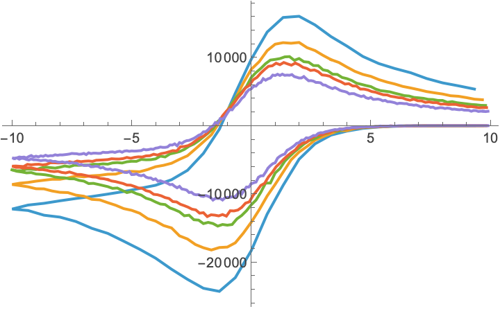
As predicted, the faster scan rates (blue) have a larger peak current:
ListLinePlot@ MapThread[Transpose[{#1, #2}] &]@ {expts, obs}
Extract the peak currents (using a Gaussian blurring at the scale of 5 adjacent elements in the list) in the oxidation and reduction directions:
peakOxCurrent = (Last@ Last@ FindPeaks[#, 5])& /@ obs

(*{16038, 12167, 10125, 9260, 7548}*)
peakRedCurrent = -(Last@ Last@ FindPeaks[-#, 5])& /@ obs (*multiply by -1 to find min*)

(*{5359, 3796, 2961, 2610, 2061}*)
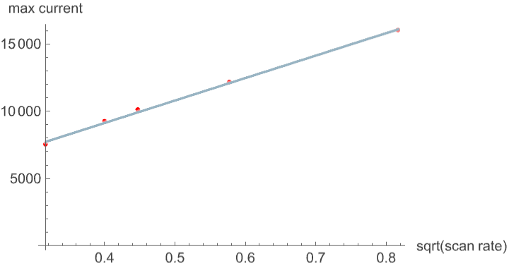
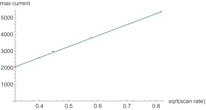
The Randles-Ševčík equation predicts that the peak current (for both the oxidation and reduction curves) is proportional to the square root of the scan rate (with different constants). The fit is pretty good for both oxidation and reduction peak currents:
Transpose[{Sqrt[rates], peakOxCurrent}];
ModelFit[%, "Linear"]
ListPlot[%%, PlotFit -> %,
  PlotStyle -> Red, AxesLabel -> {"sqrt(scan rate)", "max current"}]

Transpose[{Sqrt[rates], peakRedCurrent}];
ModelFit[%, "Linear"]
ListPlot[%%, PlotFit -> %,
  PlotStyle -> Red, AxesLabel -> {"sqrt(scan rate)", "max current"}]

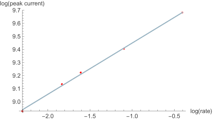
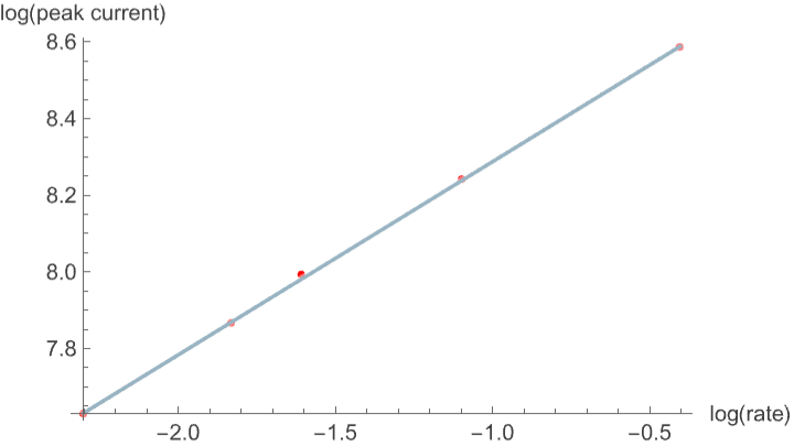
For a diffusion-controlled process, the slope of the fit of log(scan rate) and log(peak current) should be about 0.5; in our idealized simulation this is the case and we obtain approximately this exact result measuring either the oxidation or reduction:
N@Log@Transpose[{rates, peakOxCurrent}];
ModelFit[%, "Linear"]
ListPlot[%%, PlotFit -> %,
  PlotStyle -> Red, AxesLabel -> {"log(rate)", "log(peak current)"}]

N@Log@Transpose[{rates, peakRedCurrent}];
ModelFit[%, "Linear"]
ListPlot[%%, PlotFit -> %,
  PlotStyle -> Red, AxesLabel -> {"log(rate)", "log(peak current)"}]

Gratuitous Chiguiro Content
Chiguiros are not very good at remembering equations:
ImageSynthesize["Capybara explaining the Randles-Ševčík equation"]

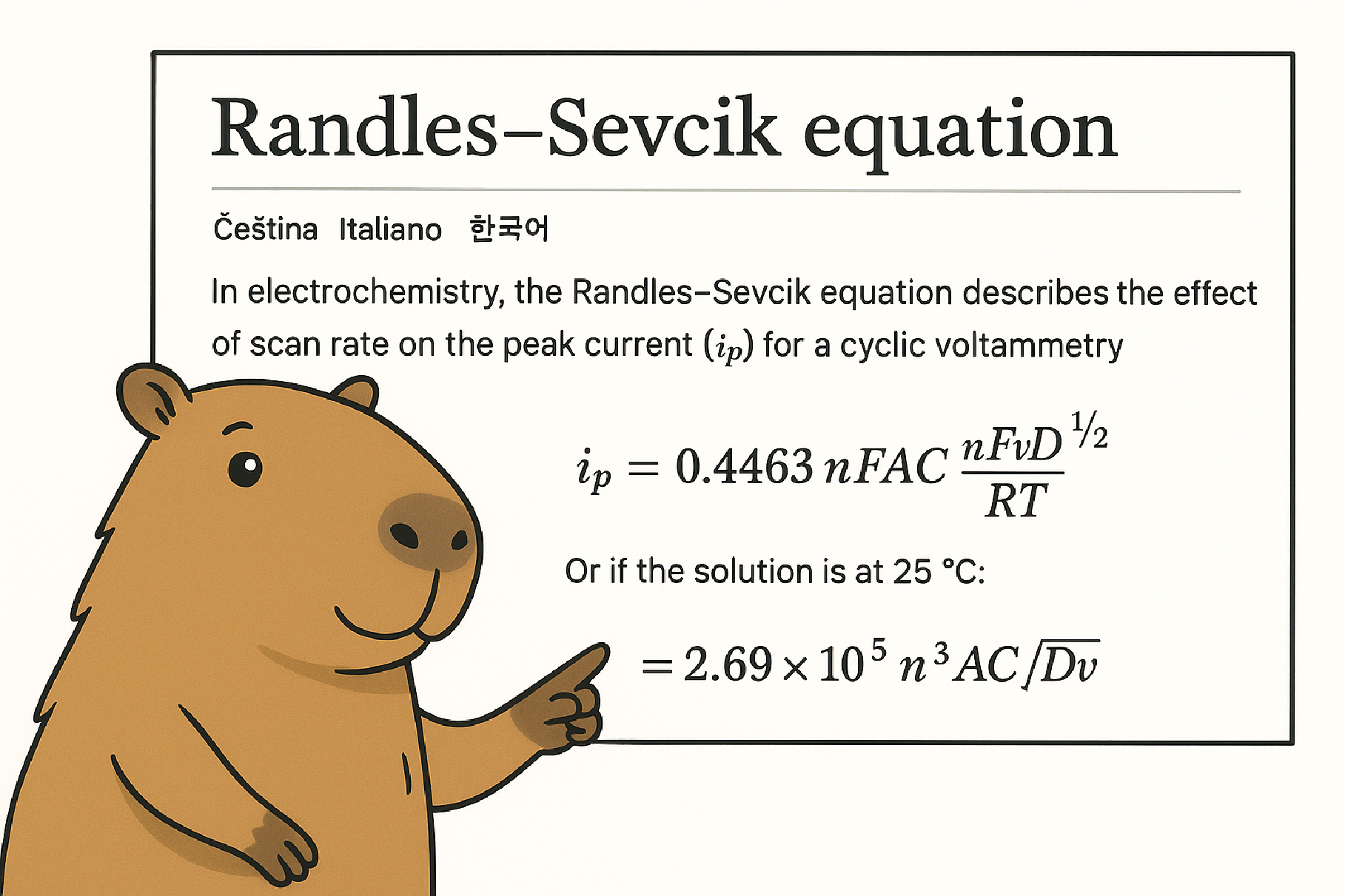
But they can look things up on the internet:
ImageSynthesize["Capybara explaining the following wikipedia page" <>
  Import["https://en.wikipedia.org/wiki/Randles-Sevcik_equation"]]
Remember to tell them to dress properly to deliver their lecture:
ImageSynthesize[
  "Capybara wearing a bowtie, glasses, and a tweed jacket explaining the following wikipedia page" <>
  Import["https://en.wikipedia.org/wiki/Randles\[Dash]Sevcik_equation"]]

ToJekyll["Simulated Electrochemistry, part 2", "chemistry mathematica montecarlo science teaching electrochem"]
Monte Carlo Simulations of Electrochemistry
- Part 1: Monte Carlo Simulation of Diffusion, Chronoamperometry, Linear & Cyclic Voltammetry
- Part 2: Reproducing the Randles–Ševčík Relation — this post
- Part 3: Irreversible Cyclic Voltammetry and Quantification
- Part 4: Anodic Stripping Voltammetry
- Part 5: Optimizing the Monte Carlo Simulation
- Part 6: Concentration Profiles During Cyclic Voltammetry