Simulated Electrochemistry, part 3: Irreversible CV
[chemistry mathematica montecarlo science teaching electrochem chiguiro In our previous episodes, we implemented Monte Carlo simulations of chronoamperometry and voltammetry, and showed how the simulated current dependence on scan rate reproduces the Randles-Ševčík equation. In this post, we adapt this code to simulate an irreversible cyclic voltammetry experiment for concentration determination….
Motivating Experiment
Chiguiros (like humans, guinea pigs, and a few other species) lack the L-gulonolactone oxidase enzyme needed to synthesize their own vitamin C, and thus must consume about 1000mg/day to avoid scurvy. A classic way to determine ascorbic acid concentration is to measure the peak current during irreversible oxidation by cyclic voltammetry. To simulate this, we will need to adapt our previous Monte Carlo simulation code to model an irreversible process. We will also need to properly account for concentration effects in the simulation. The desired outcome is to simulate the type of calibration standard curve that one would make in the laboratory.
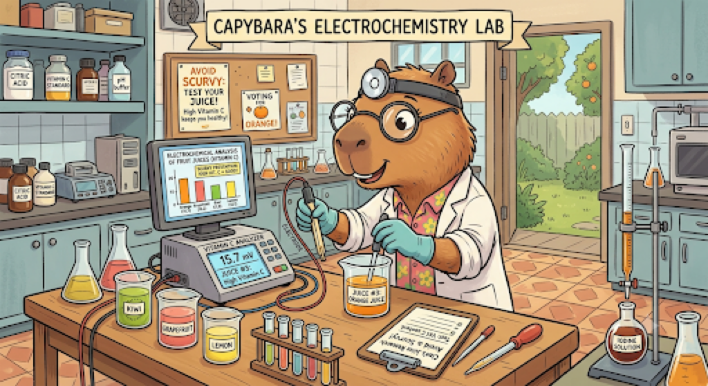
(image courtesy of BoB the Chemist)
Computational Methods
We can simply reuse the cyclic voltammetry profile generator function from last time:
cv[v0_, time_Integer] := With[
   {v = N@Rest@Subdivide[v0, -v0, time/2] },
   Join[v, Rest@Reverse[v]]]
Small modifications are required to the Monte Carlo simulation code. Specifically, to model the ascorbic acid problem we start in the reduced state rather than the oxidized state. Because it is an irreversible process, once the molecule has been oxidized, it cannot go back to the reduced state:
irreversibleF = FunctionCompile@Function[
    {Typed[vv, TypeSpecifier["PackedArray"]["Real64", 1]],
     Typed[maxX, TypeSpecifier["Integer16"]]},
    Module[
     {x =  RandomInteger[{1, maxX}],
      state = -1,                                     (*!! start in reduced state: ascorbic acid *)
      obs = ConstantArray[0, Length[vv]],
      dx = 2 RandomInteger[{0, +1}, Length[vv]] - 1},
     Do[
      x += dx[[t]];
       If[x == 0,
        If[RandomReal[] < 1./(1. + Exp[-vv[[t]]]),
         If[state == -1, obs[[t]] = +1; state = +1;], (*!! oxidized into dehydroascorbic acid *)
         If[state == +1, Null;]                       (*!! do nothing, the reaction is irreversible *)
        ];
        x = 1;
       ];
      , {t, Length[vv]}];
     obs
    ]]

(One could entirely remove the If[state ==+1, Null;], but leaving it in serves as a mental reminder to the scientific programmer that the possibility has been considered and is deliberately not being actioned upon. )
Results and Discussion
Begin by defining the voltage profile as a function of time for the experiment; here, we perform the sweep in the opposite direction as before (from negative to positive):
expt = cv[-10., 400]; (* sweep from negative to positive *)
As you will recall from our previous discussion of the Randles-Ševčík equation, the simulated concentration is proportional to the number of Monte Carlo trials divided by the magnitude of the sampling region. Thus for some maximum concentration we might define the sampling region as extending to Ceiling[6 Sqrt[d t]] as before, and then for smaller concentration we increase the size by dividing by the concentration–essentially we are diluting the reactive species.
To get good statistics, we will run each simulation for 10^7 trials. Rather than run the calculation locally, we can use RemoteBatchMapSubmit to dispatch these calculations to a remote server. For a short (few minutes) calculation like this, it does not save us much time, but it does allow us to work on the subsequent plots, etc. without tying up the local kernel:
maxConc = Ceiling[6*Sqrt[0.5*400]];
concentrations  = {1.0, 0.9, 0.8, 0.6, 0.5, .25, .1};

jobs = RemoteBatchMapSubmit[ (* ...or just use Map to run locally *)
   ParallelSum[irreversibleF[expt, #], {i, 10^7}] &,
   Round[(maxConc/concentrations)]]

Keep an eye on the job status with a live update (of course, now that I am writing this, the jobs have all completed); I was surprised that it dispatched this to 3 jobs rather than 7, but I assume this choice was made by accounting for the job startup overhead:
jobs["DynamicStatusVisualization"]

When the jobs are completed, retrieve the observed results (a vector of observed currents at each timestep) and plot the simulated voltammograms for each of the initial concentrations:
obs = jobs["EvaluationResults"];

ListLinePlot[
  Map[Transpose[{expt, #}] &]@ obs ,
  PlotStyle -> ColorData[40, "ColorList"],
  PlotLegends -> Placed[concentrations, {Left, Top}],
  Frame -> True, FrameLabel -> {"nF(E-E')/RT", "current"}]
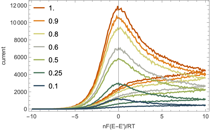
Unlike the reversible process, we observe only a single oxidation peak for each simulation (and no reduction peak) and the peak is located directly over the formal potential of our analyte (which we have set as our zero). The peak current (number of events) appears to be proportional to the concentration.
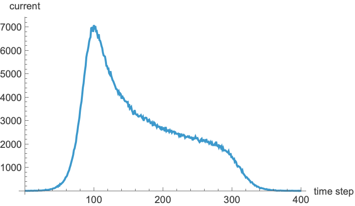
It will be more useful to work with the direct output of current as a function of time, for example:
ListLinePlot[obs[[4]], AxesLabel -> {"time step", "current"}]
Extract the peak current value, using a Gaussian blur of 10 timesteps to remove noise, from each of the simulated observations; each should have one global maximum which is the first local maximum:
peakCurrent = (Last@First@FindPeaks[#, 10]) & /@ obs

(*{11922, 10729, 9442, 7046, 5839, 2958, 1210}*)
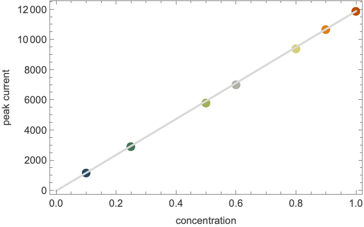
Generate the standard curve by plotting concentration versus peak current:
data = Transpose[{concentrations, peakCurrent}];
model = ModelFit[data, "Linear"]

Show[
  ListPlot[
   List /@ data,
   PlotStyle -> ColorData[40, "ColorList"],
   PlotMarkers -> {"\[FilledCircle]", Medium},
   Frame -> True, FrameLabel -> {"concentration", "peak current"}],
  Plot[model[x], {x, 0, 1}, PlotStyle -> LightGray]]

Peer Review
BoB The Chemist notes:
The pedantic electrochemist would specify chemically irreversible due to the coupled chemical reaction. I’m also a bit suspicious about the return feature shape. See for example here PSAN0201-Vitamin-C-Detection-with-ItalSens-Carbon-SPE.pdf The return feature has a more pronounced sigmoidal shape than what I see in your Sims. This might be due to radial vs linear diffusion.
ImageSynthesize["A capybara working as an old-time newspaper copy editor with a green visor reviewing documents. Do not include any text."]

Conclusion
We have successfully modeled a chemically irreversible CV experiment, and the simulated peak currents show the ideal linear relationship to concentration that would be needed to quantify an unknown concentration.
What does a chiguiro think about this? Chiguiros have high social intelligence, but are challenged by complex cognitive tasks. As we can see in the image below, they still struggle to distinguish between irreversible and reversible processes even after reading this post.
ImageSynthesize["A capybara typing on a 1980s classic Macintosh desktop computer, on the screen of the computer is an image of the irreversible cyclic voltammogram of ascorbic acid oxidation"]

ToJekyll["Simulated Electrochemistry, part 3: Irreversible CV",
  "chemistry mathematica montecarlo science teaching electrochem chiguiro"]
Monte Carlo Simulations of Electrochemistry
- Part 1: Monte Carlo Simulation of Diffusion, Chronoamperometry, Linear & Cyclic Voltammetry
- Part 2: Reproducing the Randles–Ševčík Relation
- Part 3: Irreversible Cyclic Voltammetry and Quantification — this post
- Part 4: Anodic Stripping Voltammetry
- Part 5: Optimizing the Monte Carlo Simulation
- Part 6: Concentration Profiles During Cyclic Voltammetry