Distributed data storage with libSQL
[science claude-light sdl ml teaching mathematica sql In our previous episode, we showed how to specify an experiment and retrieve the results from a claude-light device over HTTP, and then used active learning to construct a digital twin model of the outputs. In this episode we will explore the use of libsql, a new, cloud-native rewrite of sqlite, that will enable distributed data sharing by sharing access tokens….
(this is largely my thinking through notes originally composed by Prof. John Kitchin, translating them into Mathematica, and editorializing on the process and code)
Pre-reqs
We assume basic knowledge of the unix command line — creating files, changing directories, and running commands
LibSQL Database Setup
-
Begin by getting a free account at [https://turso.tech]
-
Install the turso CLI and then create a database using the following commands from your terminal window:
turso auth login
turso db create claude-light
- Create a file named setup.sql with the following contents:
CREATE TABLE IF NOT EXISTS
  measurements (
    id INTEGER PRIMARY KEY,     -- this is the rowid
    data JSON                   -- JSON blob (stored as TEXT under the hood)
  )
- From a terminal window, run the following command to setup the database schema for your database (in principle, you can execute arbitrary commands in this way):
turso db shell claude-light <setup.sql
- As mentioned in the introduction, LibSQL/Turso allows you to have a local copy of the database which is synced to a cloud copy. Furthermore, you give other people read+write or read-only access to the cloud version by providing them with an access token (this is like an API key). To find out what the URL and tokens are, run the following commands in the terminal window:
turso db show --url claude-light
turso db tokens create claude-light
turso db tokens create claude-light -r
We want to save these for use later on. As we will be doing this in Mathematica, the best way is to define SystemCredential values for each of these. From here onward we run all commands in Mathematica:
SystemCredential["CLAUDELIGHT_DB_URL"] = "libsql://claude-light-jschrier.aws-us-east-1.turso.io"

SystemCredential["CLAUDELIGHT_RW"] = (* redacted *);

SystemCredential["CLAUDELIGHT_RO"] = "eyJhbGciOiJFZERTQSIsInR5cCI6IkpXVCJ9.eyJhIjoicm8iLCJpYXQiOjE3NTM5ODI3NzQsImlkIjoiMmI5MzFiMGUtOWFhYS00MDMzLWE1YjAtYmI0MzU3YWMxYmUzIiwicmlkIjoiYTY3MTZiNjUtMTA5OC00NjdiLTkwYTgtYWQ5MmIyNTE1ZGU4In0.MYY6LeIEUQYsjxcvAStV9dZBaBWE0gyl6JpqN4DPltyALt0ho-J8z3i_MemBb7gRuxXKdKp8pOOswYAOmq8ZAA"
Turning our measurement into a JSON object
Previously, we defined a HTTP GET request that retrieved the experimental outputs for a given input:
measurement[{r_, g_, b_}] :=
   URLExecute["https://claude-light.cheme.cmu.edu/api", {"R" -> r, "G" -> g, "B" -> b}]

 (* demo *)
example = measurement[{0.1, 0.2, 0.3}]

(* {"in" -> {0.1, 0.2, 0.3},
   "out" -> {"415nm" -> 913, "445nm" -> 9882, "480nm" -> 5764, "515nm" -> 14199,
             "555nm" -> 3524, "590nm" -> 3492, "630nm" -> 5071, "680nm" -> 2208,
             "clear" -> 30658, "nir" -> 3967}} *)
We will convert this data structure into a JSON representation string for insertion into the database:
ExportString[example, "JSON"]

(*"{	\"in\":[		0.1,		0.2,		0.3	],	\"out\":{		\"415nm\":913,		\"445nm\":9882,		\"480nm\":5764,		\"515nm\":14199,		\"555nm\":3524,		\"590nm\":3492,		\"630nm\":5071,		\"680nm\":2208,		\"clear\":30658,		\"nir\":3967	}}"*)
But let us take one step further to also include relevant metadata (who/what/when/where/why/how information) about the experiment and prepend that to our exported result:
metadata[versionedFunction_String, tag_ : Null] := With[
    {functionCode = ToString@ InputForm@FullDefinition[versionedFunction]},
    {"version" -> Hash[functionCode, "SHA256", "HexString"],
     "func" -> functionCode,
     "t0" -> AbsoluteTime[],
     "user" -> $Username,
     "hostname" -> $MachineName,
     "tag" -> tag}]

measurementJSON[{r_, g_, b_}, tag_ : Null] := With[
    {meta = metadata["measurementJSON", "tutorial"],
     data = measurement[{r, g, b}]},
    ExportString[Join[meta, data], "JSON", "Compact" -> 1]]

 (*demo*)
(example = measurementJSON[{0.1, 0.2, 0.3}, "tutorial"]) // Rasterize
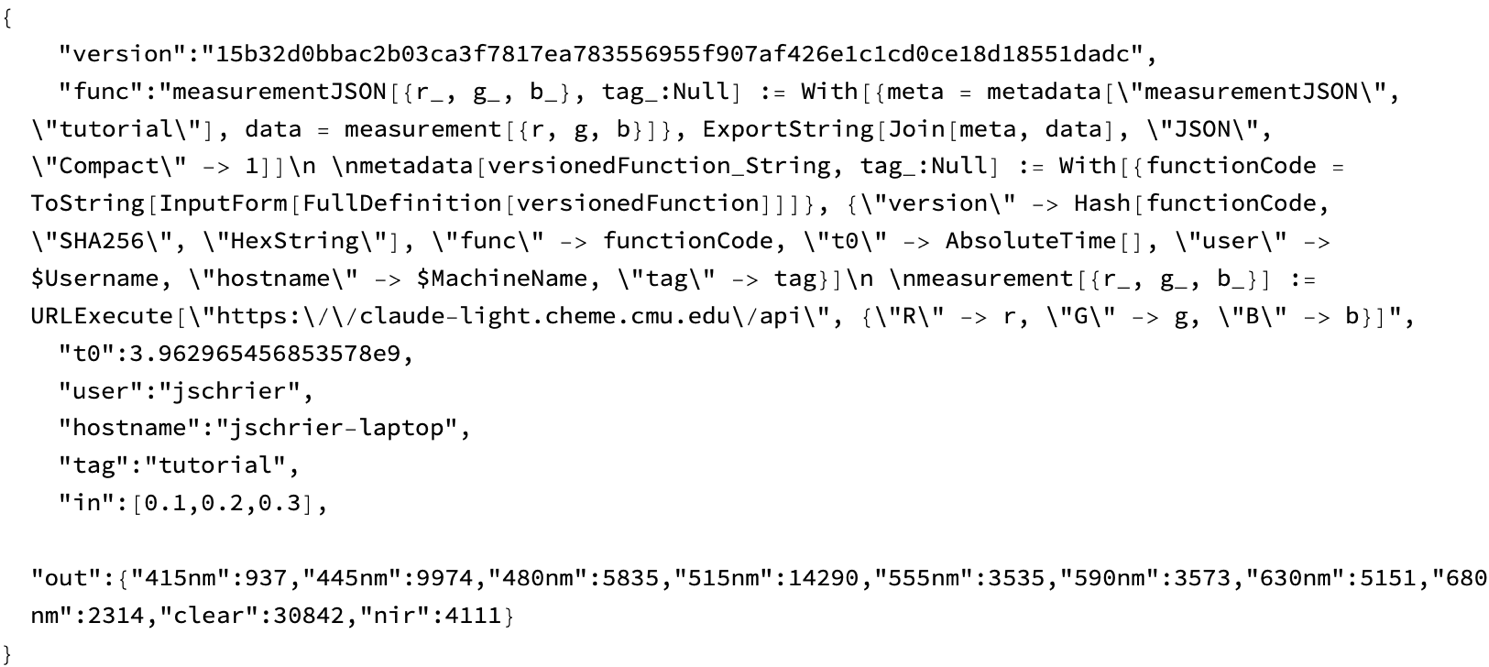
(Observe that there is some advanced trickery in the metadata function, especially in the use of FullDefinition to the definitions of all symbols that the named function depends upon. By appending the code text and a SHA digest into the JSON we can track the how aspects of the experiment, although this type of brute force way will waste a lot of space in our database in a production setting.)
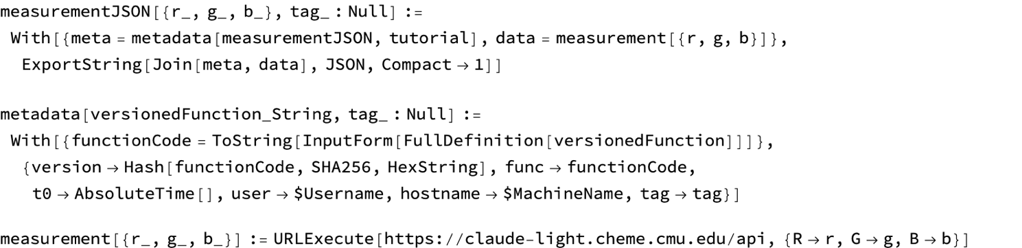
FullDefinition["measurementJSON"] // Rasterize
Interacting with the libSQL database in Mathematica
We will programmatically interact with the database in 4 ways:
-
connect: This function is used to connect to the database and establish syncing with the remote version (given the proper authorization token). This is done at the beginning of a session.
-
execute: This function is used to run SQL statements. You can use it to perform both read and write operations. It can be invoked with a SQL statement as a string or an object, and it supports placeholders for parameterized queries.
-
commit: A process might involve multiple SQL statements which would be incomplete on their own; you can execute them all, and then when everything is ready commit to permanently save the changes into the database.
-
sync: This function, unique to libSQL, synchronizes a local database with a remote counterpart. It ensures that the local database is updated with the latest changes from the remote database. This is particularly useful when working with embedded replicas or when you need to ensure data consistency across distributed environments. (Note that it is also possible to enable periodic automatic syncing when initializing the connection.)
Turso/libSQL provides a python API, and while our code of conduct does not forbid us from using such uncivilized resources when required, to preserve some semblance of dignity we shall run Python solely through Mathematica as an interface. Admittedly this is a bit ugly, as we are trying to map the python object-oriented programming model into a functional style term substitution system.
Begin by creating a python virtual environment session with the required library and import it:
session = ResourceFunction["StartPythonSession"][{"libsql"}]
ExternalEvaluate[session, "import libsql"]

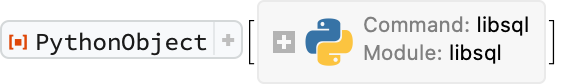
Then, create the object we will use:
libsql = ResourceFunction["PythonObject"][session, "libsql"]
We use object as we would in python, but [ replaces the . and ( characters for denoting methods and their argument indicators:
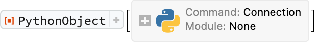
conn = libsql["connect"["claude_light.db",
    "sync_url" -> SystemCredential["CLAUDELIGHT_DB_URL"],
    "auth_token" -> SystemCredential["CLAUDELIGHT_RW"]]]
conn["sync"[]]
The presence of sync at the the end synchronizes our local database with the cloud version at the sync_url.
Values are inserted by executing SQL commands with the execute function. For now we will merely concatenate our JSON example string into this command (later we will write a wrapper function). After performing some number of SQL commands, we then commit them to the local database and then sync with the remote database.:
conn["execute"["INSERT INTO measurements(data) VALUES ('" <> example <> "');"]]
conn["commit"[]]
conn["sync"[]]
Values are also read from the database by using execute to perform a SQL select query:
cursor = conn["execute"["select * from measurements"]]

The cursor object (which we have saved into a variable named cursor) has several functions we can call:
cursor["Information"]

(* <|"Methods" -> {},
    "Builtins" -> {"close", "execute", "executemany", "executescript", "fetchall", "fetchmany", "fetchone"},
    "ClassVariables" -> {"rowcount", "lastrowid", "arraysize", "description"},
    "InstanceVariables" -> {"__init__"}|> *)
fetchall returns a (Mathematica) list of all of the data…in this case, the one entry we have added so far:
cursor["fetchall"[]]

(*{ {1, "{	\"version\":\"15b32d0bbac2b03ca3f7817ea783556955f907af426e1c1cd0ce18d18551dadc\",	\"func\":\"measurementJSON[{r_, g_, b_}, tag_:Null] := With[{meta = metadata[\\\"measurementJSON\\\", \\\"tutorial\\\"], data = measurement[{r, g, b}]}, ExportString[Join[meta, data], \\\"JSON\\\", \\\"Compact\\\" -> 1]]\\n \\nmetadata[versionedFunction_String, tag_:Null] := With[{functionCode = ToString[InputForm[FullDefinition[versionedFunction]]]}, {\\\"version\\\" -> Hash[functionCode, \\\"SHA256\\\", \\\"HexString\\\"], \\\"func\\\" -> functionCode, \\\"t0\\\" -> AbsoluteTime[], \\\"user\\\" -> $Username, \\\"hostname\\\" -> $MachineName, \\\"tag\\\" -> tag}]\\n \\nmeasurement[{r_, g_, b_}] := URLExecute[\\\"https:\\/\\/claude-light.cheme.cmu.edu\\/api\\\", {\\\"R\\\" -> r, \\\"G\\\" -> g, \\\"B\\\" -> b}]\",	\"t0\":3.962965456853578e9,	\"user\":\"jschrier\",	\"hostname\":\"jschrier-laptop\",	\"tag\":\"tutorial\",	\"in\":[0.1,0.2,0.3],	\"out\":{\"415nm\":937,\"445nm\":9974,\"480nm\":5835,\"515nm\":14290,\"555nm\":3535,\"590nm\":3573,\"630nm\":5151,\"680nm\":2314,\"clear\":30842,\"nir\":4111}}"}}*)
Given how often we might do this, we might streamline this process by putting these operations together:
conn["execute"["select * from measurements"]]["fetchall"[]]
Now that we have seen the basic mechanics, it is a good time to streamline this process by defining some convenience functions:
execute[connection_, command_String] := connection["execute"[command]]
commit[connection_] := connection["commit"[]]
sync[connection_] := connection["sync"[]]
fetchall[cursor_] := cursor["fetchall"[]]

insertMeasurement[connection_, item_String] := With[
   {cmd = StringTemplate["INSERT INTO measurements(data) VALUES ('``');"]},
   execute[connection, cmd[item]];
   commit[connection];
   sync[connection];]
Use this to add another example or two to our database:
With[
  {m = measurementJSON[{0.4, 0.5, 0.6}, "tutorial"]},
  insertMeasurement[conn, m]]
Retrieving Data
When it comes time for analysis, we can use the SQL SELECT command to search through the data. Conveniently SQLite (and by extension, libSQL) allows us to perform direct database queries on the JSON text that we have stored. This is certainly convenient, although computationally more time-consuming than creating a proper schema.
results = fetchall@execute[conn, "SELECT * FROM measurements WHERE json_extract(data, '$.tag') = 'tutorial'"];
This will return a list of JSON strings, so read them into a more reasonable format, and make a nice plot of the output values:
Dataset@ Query[All, "out"]@ Map[ImportString[#, "RawJSON"] &]@ results[[All, 2]]
We may as well make a convenience function for this:
queryMeasurements[connection_, query_String] := With[
   {cmd = StringTemplate["SELECT * FROM measurements WHERE ``;"]},
   Map[ImportString[#, "JSON"] &]@#[[All, 2]] &@fetchall@execute[connection, cmd[query]]]
Apply to selecting on other data:
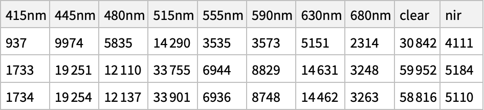
 Query[All, {"in", "out"}]@queryMeasurements[conn, "json_extract(data, '$.in') = '[0.4,0.5,0.6]'"]

(*{ { {0.4, 0.5, 0.6}, {"415nm" -> 1733, "445nm" -> 19251, "480nm" -> 12110, "515nm" -> 33755, "555nm" -> 6944, "590nm" -> 8829, "630nm" -> 14631, "680nm" -> 3248, "clear" -> 59952, "nir" -> 5184}}, { {0.4, 0.5, 0.6}, {"415nm" -> 1734, "445nm" -> 19254, "480nm" -> 12137, "515nm" -> 33901, "555nm" -> 6936, "590nm" -> 8748, "630nm" -> 14462, "680nm" -> 3263, "clear" -> 58816, "nir" -> 5110}}}*)
Read-only analysis
We can always create a read-only session using the same approach and then query for data of interest. The only difference is using the read-only token:
roConn = libsql["connect"["claude_light.db",
      "sync_url" -> SystemCredential["CLAUDELIGHT_DB_URL"],
      "auth_token" -> SystemCredential["CLAUDELIGHT_RO"]]];

Query[All, "out", "630nm"]@queryMeasurements[roConn, "json_extract(data, '$.tag') = 'tutorial'"]

(*{5151, 14631, 14462}*)
Bonus: Initializing the Database
We could have created the database schema programmatically by using an execute command!
execute[conn,
  "create table if not existsmeasurements (id   INTEGER PRIMARY KEY,  -- this is the rowiddata JSON                 -- JSON blob (stored as TEXT under the hood))"]
sync[conn]
Closing connections
It is always a good idea to close your database (even if many tutorials do not include this):
conn["close"[]]
And also useful to end the python session within your Mathematica notebook (although also not strictly necessary)
DeleteObject[session]
Next steps
-
Saving steps taken during an Active Learning run into the database as we go along
-
Incorporate side information into the model (time of day, sun position, is it during working hours, etc.) into the predictive model
ToJekyll["Distributed data storage with libSQL", "science claude-light sdl ml teaching mathematica sql"]