Controlling a remote lab and using active learning to construct digital twin model

John Kitchin recently described Claude-Light (a REST API accessible Raspberry Pi that controls an RGB LED with a photometer that measures ten spectral outputs) as a lightweight, remotely accessible instrument for exploring the idea of self-driving laboratories. Here we demonstrate how to implement a very basic active learning loop using this remote instrument in Mathematica…

Backstory

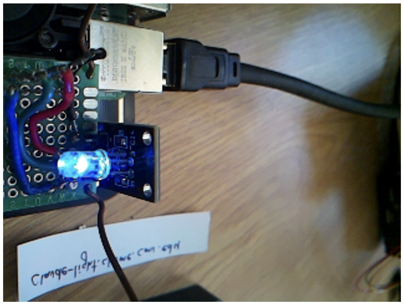
The idea of an autonomous experiment systems (AES) or self-driving laboratory (SDL) has fascinated me since my participation in the 2017 Materials Acceleration Platform report and continues to this day. This is now a major field with large investments made throughout the world(1)(2). But if we want this emerging field to be accessible to researchers (and students!) then frugal SDLs are needed. The cheapest reagents are photons, and so there are various light-based SDL projects intended for teaching, in which the experimental input is the setting of an RGB LED and the output is a colorimetric response, of which Claude-Light is the latest example. What sets it apart is that it is web-accessible, so that students operate the hardware and obtain measurements remotely. The sensors are deliberately not shielded from ambient light in the office, so in addition to the inherent measurement noise of the sensors there will also be other variations that occur independent of the LED setting (not unlike how uncontrolled changes in ambient lab humidity can affect crystallization outcomes).

Here is what it looks like:

One general strategy in automated science is acquiring data from an instrument and building a digital twin (i.e., a machine learned model of a physical system) that predicts the output values for a given input. In typical supervised machine learning you have a bunch of pre-obtained data and must construct a model. However, if you can tell the SDL what new data to acquire (i.e., what experiment to perform) then you can instead perform active learning improve the model quality with fewer experiments. We have previously applied active learning to various problems such as perovskite crystal growth (including a bakeoff-style competition of various methods) and nanocrystal ligand selection.

Goal: Demonstrate how to read data from a remote Claude-Light and how to train and evaluate an active learning model using that data, in the Wolfram language.

Claude-Light

• You can read all about it in the Claude-Light paper (including a basic usage tutorial in Python)

• Or just go over to the github repository and check out some example exercises.

• Or just hop on the instrument web site and start banging on it a bit to get some intuition.

Acquiring Values from Claude-Light

We do not want to manually acquire data…we want our program to do it for us. Conveniently, Claude-Light exposes a REST API that we can use to acquire data by performing an HTTP GET call. We shall do this by using a simple URLExecute to provide the URL and parameters. (Should you want to perform more complicated HTTP requests, or build in error handling, you would first construct a HTTPRequest and then evaluate that, check error messages, etc. We shall keep it simple here.) Our input is a triple of RGB values provided as real numbers between 0 and 1:

measurement[{r_, g_, b_}] := 
  URLExecute["https://claude-light.cheme.cmu.edu/api", {"R" -> r, "G" -> g, "B" -> b}]

Take a look at an example:

measurement[{0.1, 0.2, 0.3}]

(*
{"in" -> {0.1, 0.2, 0.3}, 
 "out" -> {"415nm" -> 1549, "445nm" -> 11055, "480nm" -> 7418, "515nm" -> 16576, 
  "555nm" -> 6108, "590nm" -> 6556, "630nm" -> 8111, "680nm" -> 5982, "clear" -> 46032, "nir" -> 7787}}
*)

We are going to focus our model on learning one wavelength, so let us Query this output to see what happened at that one wavelength:

measure445nm[in_] := Query["out", "445nm"]@ measurement@ in

Active Learning in Mathematica

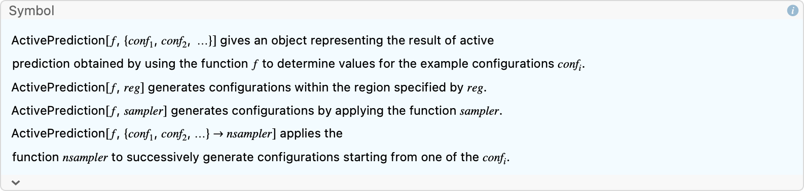
One could just perform standard supervised machine learning: query a bunch of random samples, organize them into a table, and then build a machine learning model to describe the input-output behaviour using Predict. But the more efficient active learning approach is to let our model select the next sample to query based on the model uncertainty at each step. The ActivePrediction superfunction will iteratively query a function, f, to attempt to learn an approximation, trying different machine learning methods along the way. In our case, f will be the measure445nm function defined above.

?ActivePrediction

The default options are mostly reasonable:

Options[ActivePrediction]

(* {ClassPriors -> Automatic, FeatureExtractor -> Identity, FeatureNames -> Automatic, FeatureTypes -> Automatic, IndeterminateThreshold -> 0, InitialEvaluationHistory -> None, “InitialEvaluationNumber” -> Automatic, MaxIterations -> Automatic, Method -> “MaxEntropy”, PerformanceGoal -> Automatic, RandomSeeding -> 1234, “ShowTrainingProgress” -> True, TimeConstraint -> [Infinity], UtilityFunction -> Automatic, ValidationSet -> Automatic} *)

Notice how the default method chooses new configurations (i.e., RGB points) for which the learned predictor function has the maximum uncertainty. (It is possible to specify a particular model choice with the Method option, and indeed, we expect LinearRegression to work fine for this type of problem, but we will let ActivePrediction figure it out for us.) Note also how RandomSeeding is automatically specified for better reproducibility. We will limit the number of function evaluations (MaxIterations), but it may also be useful to set a TimeConstraint (this will be the time needed to acquire the data and build the models).

Active Learning

In practice, this is simple; it could be a one-liner, but I shall comment each input argument to the function:

result = ActivePrediction[
   measure445nm,        (* function to call to request a sample *)
   Cuboid[],            (* boundary of input: Unit cube from [0,1] on 3 axes *)
   MaxIterations -> 25] (* set upper bound on number of function calls allowed *)

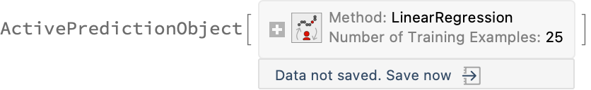
Run this and you will see some interactive progress. When completed, one can query the returned ActivePredictionObject to learn about the process and the final results:

result["Properties"]

(* {"OracleFunction", "EvaluationHistory", "Method", "Properties", "LearningCurve",
   "TrainingHistory", "PredictorFunction", "PredictorMeasurementsObject"} *)

What were the sampled input configurations and returned values?

result["EvaluationHistory"]

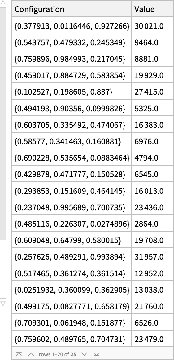
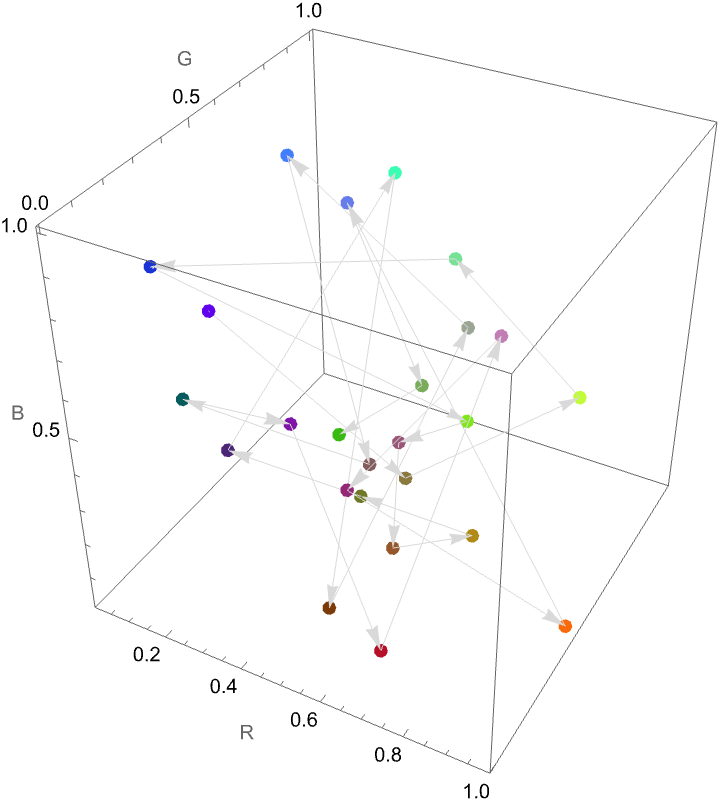
What data was acquired and in what order? (As you can see by the arrows, we bounce around the input space…)

With[
  {pts = Normal@result["EvaluationHistory"][All, "Configuration"]}, 
  Graphics3D[
   {PointSize[Large], 
    Point[pts, VertexColors -> (RGBColor @@@ pts)], 
    LightGray, Arrowheads[0.03], 
    Arrow /@ Partition[pts, 2, 1]}, 
   Axes -> True, AxesLabel -> {"R", "G", "B"}]]

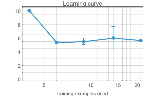
How did the model improve as we increased the number of training examples?

result["LearningCurve"]

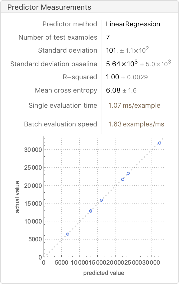
What are the summary statistics about the learned model and its performance?

result["PredictorMeasurementsObject"]

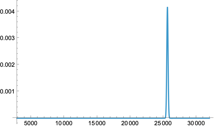
Uncertainty can be quantified by requesting a distribution description of the predicted outcome, and then work with that symbolic NormalDistribution to extract the 95%-confidence limit, plot the probability density function, etc. Let us consider a randomly generated test point in the RGB input space:

test = RandomPoint@Cuboid[]; 
 
prediction = result["PredictorFunction"][test, "Distribution"]
Quantile[%, {0.025, 0.975}] 
 
Plot[
  PDF[prediction, x], 
  Prepend[x]@ MinMax@ result["EvaluationHistory"][All, "Value"], 
  PlotRange -> All]

(*NormalDistribution[25612.5, 95.5023]*)

(*{25425.3, 25799.7}*)

In practice this prediction is pretty good and falls well within our 95% CL:

actual = output445nm[test]

(*25496*)

However…remember that by construction, Claude-Light does not isolate the sensors from the ambient environment. This means that a model that we train at noon (when sun is shining in the window and the office lights are on) will not necessarily make a good prediction at midnight (hopefully Prof. Kitchin is sleeping).

Possible Next Steps

• Saving a shareable archive of your experimental data using libSQL…see the next episode on this blog

• Incorporating side information into the model (time of day, sun position, is it during working hours, etc.)

• Explore combined meta-learning / active learning strategies for this problem

• Reframe the problem as an optimization (minimize the difference between a target output and the generated output) and optimize it iteratively using BayesianMinimization

ToJekyll["Controlling a remote lab and using active learning to construct digital twin model, part 1", "science sdl ml teaching mathematica"]