Minimal flow-matching and rectified flow model from scratch
[ml machinelearning mathematica In a previous post we looked at implementing a diffusion-based generative machine learning model from scratch. A visit with Stefano Martiniani last month convinced me that the cool kids are doing flow-matching. So, here we will make a tutorial implementation of flow-matching in Mathematica, inspired by a recent tutorial by Scott Hawley…
Why flow matching?
Flow matching (Lipman et al. 2022) (also referred to as rectified flows…they are the same…and more on this below) is a “simulation-free approach for training continuous normalizing flows based on regressing vector fields of fixed conditional probability paths”. What does that mean? We want to generate a probability distribution that matches some examples. The way we will do this is by learning an invertible “flow” (vector field) which moves samples from one distribution to another; this is different from diffusion models where the random walks don’t allow for invertibility.
Basic flow matching
Toy example: Learn a spiral
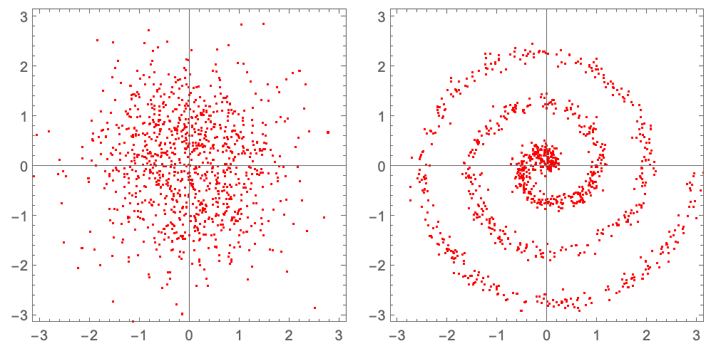
As before, we will try to learn a spiral distribution in 2 dimensions. We start from an initial state (which does not have to be a Gaussian, but it is just simple). To do this we will create some functions to generate data from each distribution (with noise) and a convenience function for plotting:
createGaussianData[nPoints_:1000, scale_:1.0] :=
   RandomVariate[NormalDistribution[], {nPoints, 2}] * scale

createSpiralData[nPoints_:1000, scale_:1.0] := With[
    {spiral = (scale/(2 Pi))*{# Cos[#], # Sin[#]}& /@ RandomReal[{0, 6 Pi}, nPoints],
     noise = 0.1*scale*RandomVariate[NormalDistribution[], {nPoints, 2}]},
    spiral + noise]

plot[data_, range_:{-Pi, Pi}] := ListPlot[ data,
   AspectRatio -> 1, PlotRange -> {range, range}, Frame -> True,
   PlotStyle -> Red, ImageSize -> Medium]
Generate source and target examples, then plot them:
source = createGaussianData[];
target = createSpiralData[];
plot /@ {source, target} // GraphicsRow
Initial Guess: Move in a Straight Line
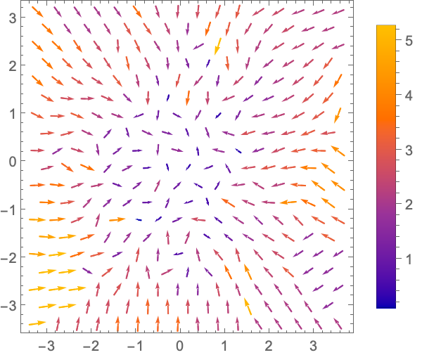
We want to learn the velocity that should be applied to each particle at each location and time. As an initial guess we will randomly pair each point in the source and target and assume that it moves in a straight line, at a constant velocity, so that it reaches the final place at after 1 unit of time. In other words, the positions at intermediate times are just a linear interpolation between the points.:
assignVelocity[source_, target_] := (target - source)
The initial velocities point every which way:
With[
  {velocities = assignVelocity[source, target]}, (* vectorized! *)
  ListVectorPlot[
   Transpose[{source, velocities}],
   VectorScaling -> Automatic, PlotLegends -> Automatic]]
Use a neural network to learn the flow field velocities.
Our goal is to learn a function that will tell us the correct velocity that a particle should move, if it is at a particular position and at a particular time between 0 and 1. (Notice the similarity with diffusion models…the main difference is there is no noise, and we are learning a deterministic function of position and time). We use a simple feed-forward neural network, with no special effort for hyperparameter design:
model[nDim_ : 2, nHidden_ : 64, activationFn_ : ElementwiseLayer["GELU"]] :=
  NetGraph[
   {NetChain[
     {AppendLayer["Input" -> nDim, "Element" -> "Real"],
      LinearLayer[nHidden], activationFn,
      LinearLayer[nHidden], activationFn,
      LinearLayer[nHidden], activationFn,
      LinearLayer[nDim]}]},
   { {NetPort["position"], NetPort["time"]} -> 1}]
untrained = NetInitialize@ model[]

Training the neural network
During model training, we will expose the model to as many locations and times as possible to cover the possible input/output space. We then force the model to learn approximately correct velocities at those locations and times that will generate our target distribution.
-
Sample random points from our source and target and pair the points.
-
Sample random times between 0 and 1.
-
Calculate the locations and velocities where these points would be at those times if they were moving at constant velocity from source to target.
-
Train the network to predict these velocities.
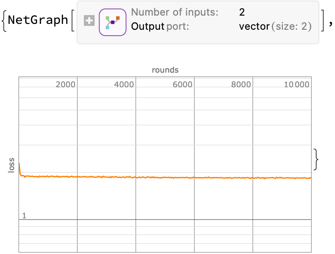
Define a sampler, and then train a neural network to minimize the mean-squared-error between the model’s prediction of the drift velocity at an interpolated position/time and the constant velocity value. We will train the heck out of it as the loss never gets particularly small:
sampler = Function[
     With[
      {source = createGaussianData[#BatchSize],
       target = createSpiralData[#BatchSize],
       time = RandomReal[{0, 1}, #BatchSize]},
      <|"position" -> (1 - time)*source + time*target,
        "time" -> time,
        "Output" -> target - source|>]];

{trained, lossPlot} = NetTrain[
   untrained, sampler,
   {"TrainedNet", "LossEvolutionPlot"},
   BatchSize -> 2048, MaxTrainingRounds -> 10000]
Evolve the particles in the learned velocity field
Next, we use the trained neural network as a velocity field to move the particles; we will do this with a simple Euler integrator:
fwdEuler[ model_, dt_][position_, time_] := With[
    {velocity = model[
      <|"position" -> position,
      "time" -> ConstantArray[time, Length[position]] |>]},
    position + velocity*dt ]

integrate[stepFn_, model_, nSteps_ : 100][source_] :=
  Fold[
   stepFn[model, 1./nSteps],
   source,
   Most@ Subdivide[nSteps]]
As one would expect, the untrained neural network is no bueno:
plot@ integrate[fwdEuler, untrained]@ source
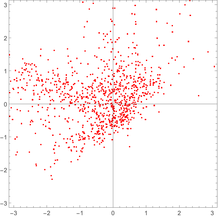
Despite the training loss function looking terrible throughout this process, the trained network does a decent job…
plot@ integrate[fwdEuler, trained]@ source
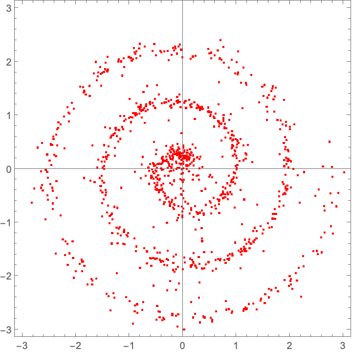
Let’s have some fun and see how it evolves in time…the infamous “collapse inward and push outward behavior”. Easy enough to do in memory; we just replace Fold with FoldList, and then ListAnimate the collection of plots:
animatedIntegrate[stepFn_, model_, nSteps_ : 100][source_] :=
   ListAnimate@ Map[plot]@ FoldList[
      stepFn[model, 1./nSteps],
      source,
      Most@ Subdivide[nSteps]]

animatedIntegrate[fwdEuler, trained]@ source
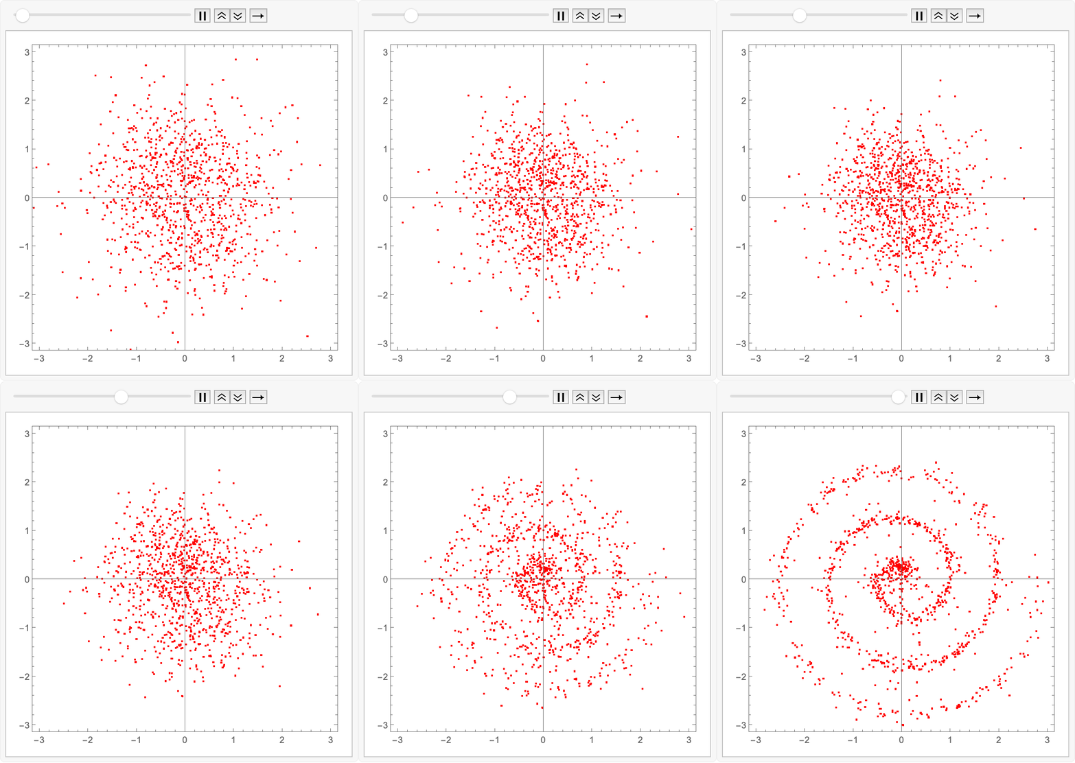
(for the readers at home…)
Export["flowmatch.gif", %];
Rectified flow (reflow) to go faster
Core idea: Instead of randomly pairing source and target points with straight line trajectories, rectified flow (Liu et al. 2023) is to use simulated targets generated by the learned flow model to predict where the particles should go, and then generate linear trajectories to those trajectories. Then use those for the linear trajectories. This straightens out the flow, which makes it faster.
 Image source: https://drscotthawley.github.io/blog/posts/images/reflow_diagram.png
This can be seen as a type of model distillation: You train a model as above to use as a teacher, and then create a new reflow model that matches that output with linear trajectories.
Upgrade 1: Time warping to add more points where needed
The animation showed that during the integration the points go inward slowly and then explode outward quickly near the end. We might do better by non-uniformly sampling time to concentrate points in the middle, where accuracy is more important. This was introduced in the Esser 2024 FLUX paper; but the specific polynomial below comes from Hawley’s tutorial. The s parameter controls the slope at t=1/2; a value of s = 0.5 is a decent choice, and s = 3/2 **approaches the cosine schedule:
warpTime[t_, s_ : 0.5] := 4 (1 - s) t^3 + 6 (s - 1) t^2 + (3 - 2 s) t

Animate[
  Plot[{warpTime[t, s], t}, {t, 0, 1},
   PlotStyle -> {Red, {Black, Dashed}}],
  {s, 0, 3/2}]
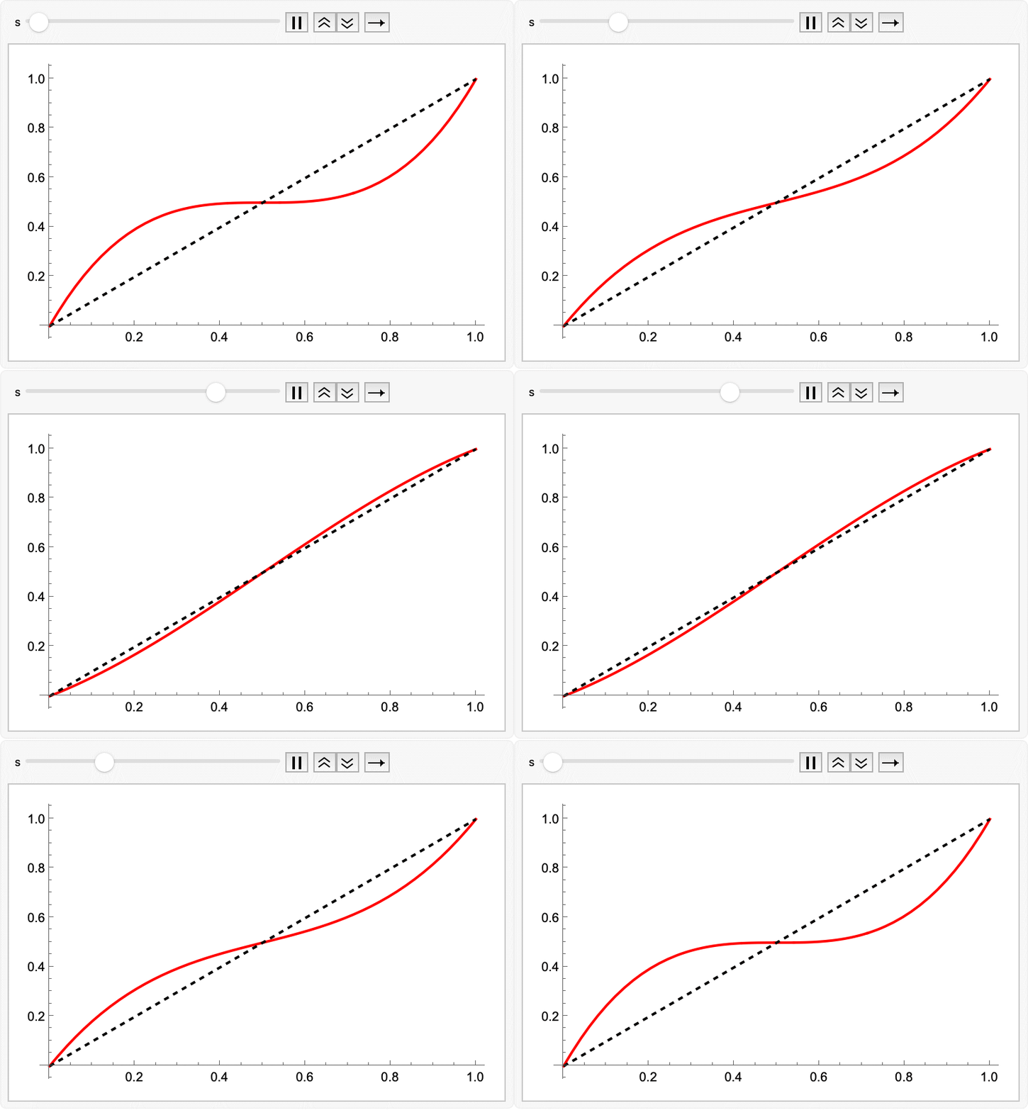
Export["timewarping.gif", %];
Note that I will only use this for adjusting the sampling, but it also common to warp the time in the integrator (however, this is even less strictly necessary).
Upgrade your Integrator to RK4
Euler integration is simple but problematic (I learned this lesson in my very first numerical algorithms course, in Fortran77, back in the day with Robert Siegfried) so use a fourth-order Runge-Kutta integrator instead. This saves a bunch of evaluations speeding up the training process (although not strictly necessary), by allowing us to to do this in fewer total steps (i.e., to take larger dt increments).
rk4[model_, dt_][x_, time_ ] := Module[
   {k1, k2, k3, k4, t},
   t = ConstantArray[time, Length[x]];
   k1 = model[<|"position" -> x, "time" -> t|>];
   k2 = model[<|"position" -> x + 0.5 dt k1, "time" -> t + 0.5 dt|>];
   k3 = model[<|"position" -> x + 0.5 dt k2, "time" -> t + 0.5 dt|>];
   k4 = model[<|"position" -> x + dt k3, "time" -> t + dt|>];
   x + (dt/6) (k1 + 2 k2 + 2 k3 + k4)]
This lets us do fewer integration steps:
plot@ integrate[rk4, trained, 20]@ source
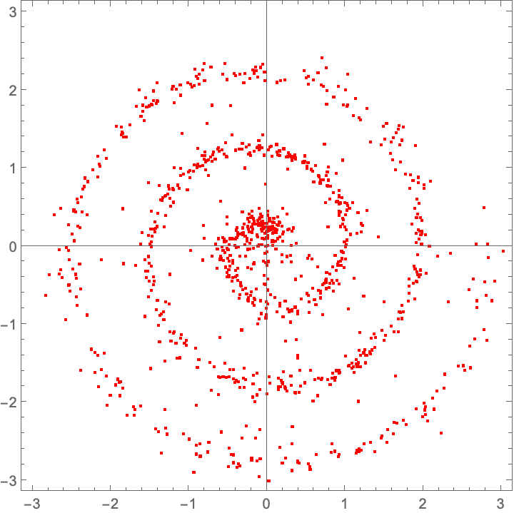
Again, not strictly necessary, but just a performance trick. As mentioned above, many people will also time-warp steps in the RK4 integration, if you see this in the wild.
We’re implementing this a function to make things easy, but this will make things a bit slower. In a production setting I would try using the Neural Network framework to perform the entire RK4 integration process for speed. Or at least try compiling a few of the intermediate steps.
Implement the reflow process
All that is left is to modify the sampler so that it uses the previously trained “teacher” neural network learned in the first part to generate hypothetical targets (integrated using our new RK4 integrator). We will also modify the sampler so that it warps time time to sample more during the middle of the trajectory. Then just go ahead a train a new network. We will start with the pre-trained network as a starting point, but it should be possible to learn a simpler network instead.
reflowSampler[teacherNet_] := Function[
    Module[{source, target, time},
     source = createGaussianData[#BatchSize];
     target = integrate[rk4, teacherNet, 20]@ source;
     time = warpTime@ RandomReal[{0, 1}, #BatchSize];
     <|"position" -> (1 - time)*source + time*target,
      "time" -> time,
      "Output" -> target - source|>]]

{reflow, lossPlot} = NetTrain[
   trained, reflowSampler[trained],
   {"TrainedNet", "LossEvolutionPlot"},
   BatchSize -> 2048, MaxTrainingRounds -> 1000]
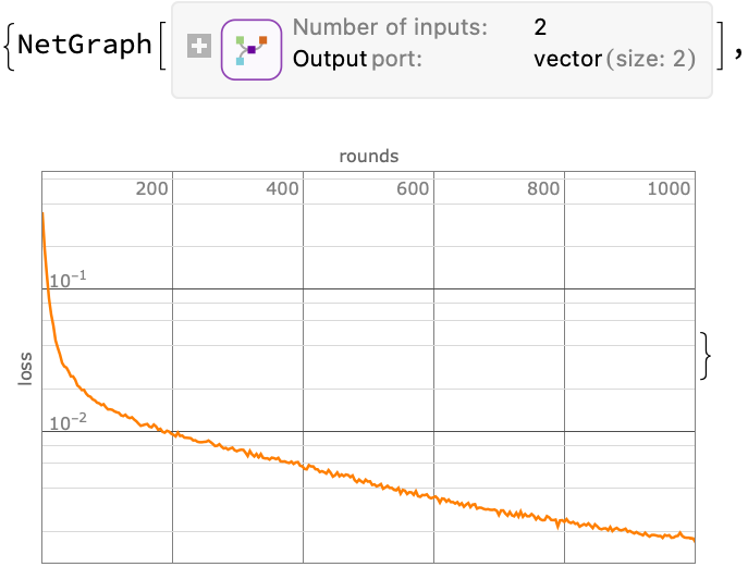
Now take a look: We do not even have to use the RK4 integrator here because the trajectories are quite simple:
animatedIntegrate[fwdEuler, reflow]@ source

Export["reflow.gif", %];
Amazing! We have indeed learned the linear-ish flow field which avoids the inward-outward velocity changes. We can compare the two approaches by just animating the two sets of exported images together:
ListAnimate@ Map[GraphicsRow]@ Transpose@ Map[Import]@
     {"flowmatch.gif", "reflow.gif"}
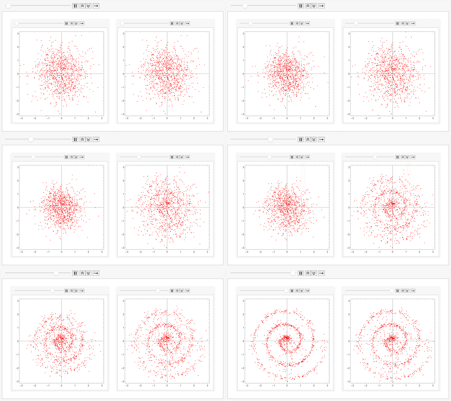
Export["combined.gif", %];
Some practical guidance/tips/observations
-
Training these models is very slow and the training loss does not give a clear sense of when to stop.
-
Notice how in the initial flow-matching required a large number of training iterations. Initial experiments with only 100 or 1000 iterations did not give good results.
-
Notice how the in the reflow example we started from the pre-trained model. Without doing this, the results were poor. Even starting from the pre-trained model and doing only 100 iterations was also poor.
-
-
Most of the time is spend on performing the integration to generate the various reflowed targets. So if you were doing this in a production setting, it would be very worthwhile to use an efficient (compiled).
ToJekyll["Minimal flow-matching and rectified flow model from scratch",
  "ml machinelearning mathematica"]
Parerga and Paralipomena
- David Koes & co. at Pitt has been working on flow-matching for molecule generation.
- Diffusion and flow-matching video course (via HN)