Minimal diffusion model from scratch for generative machine learning

Inspired by François Flueret’s post on a toy diffusion model, I decided to also explore the Ho et al. 2020 “Denoising Diffusion Probabilistic Models” paper and try to write this up as a tutorial, based on Prof. Flueret’s code. (Recently there was a post on the mathematica stack exchange which used a MNIST digit generation problem using a complicated UNet Model–for pedagogical purposes I will stick with simple 1D and 2D probability distributions to illustrate the core ideas without complicating the code.) Lilian Weng has a nice tutorial explanation of the mathematics of diffusion models that we can use as a resource, and Hugging Face has a annotated implementation tutorial in PyTorch. Diffusion models (like other generative models) convert noise into a data sample. The setup consists of two processes: (i) a fixed forward diffusion process q that gradually adds Gaussian noise to an image until it becomes pure noise; (ii) a learned reverse diffusion process p_\theta where a neural network is trained to gradually denoise an image starting from pure noise. This process is conducted over t steps. Let’s implement it!…

Toy Problems and Sample Data

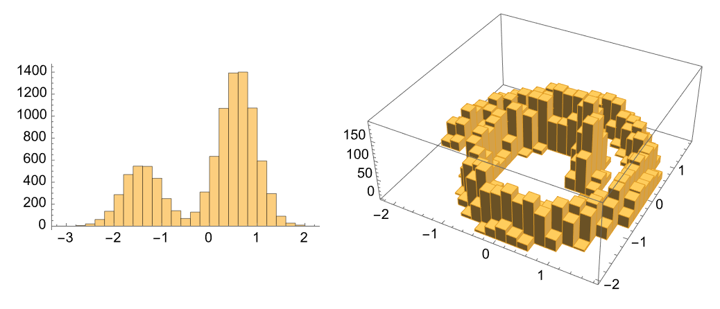
We’ll begin by defining some sample distributions that we will try to learn; they also admit higher-dimensional analogues if desired. For generality, we’ll make the input always a vector. This gets a bit awkward if it is just a vector of length one, but no matter…

sampleGaussianMixture[size_, p_ : 0.3, std_ : 0.2] := With[
    {r = RandomVariate[NormalDistribution[0, std], size]}, 
    {#} & /@ (r + Sign[RandomReal[{0, 1}, size] - p]/2)] 
 
sampleRamp[size_List] := MapThread[Min, RandomReal[{0, 1}, Prepend[2]@size]]
sampleRamp[size_Integer] := sampleRamp[{size}] 
 
sampleSpiral[size_] := With[
    {u = RandomReal[{0, 1}, size]}, 
    With[
     {rho = u*0.65 + 0.25 + 0.15*RandomReal[{0, 1}, size], 
      theta = 3*Pi*u}, 
     Transpose[{Cos[theta]*rho, Sin[theta]*rho}]]] 
  
 (*take a look*)
trainingSample1D = Standardize@sampleGaussianMixture[10^4];
trainingSample2D = Standardize@sampleSpiral[10^4];
GraphicsRow@{Histogram@Flatten@trainingSample1D, Histogram3D@trainingSample2D}

Intuitions about Forward Diffusion

Now we will try to build up the diffusion model. We’ll begin by defining functions that define some relevant constants ; in practice we’ll just include the lists that get generated into the data.

Next, we will implement the analytic expression for the diffusion process at time t.

Clear[alpha, beta, alphaBar, sigma, xt];
beta[tMax_Integer] := Subdivide[10^-4, 0.2, tMax - 1]
alpha[tMax_Integer] := 1. - beta[tMax]
alphaBar[tMax_Integer] := Exp@Accumulate@Log[alpha[tMax]]
sigma[tMax_Integer] := Sqrt@beta[tMax] 
 
xt[tMax_Integer] := With[
   {a = Sqrt[alphaBar[tMax]], 
    b = Sqrt[1. - alphaBar[tMax]]}, 
   FunctionLayer[
    a[[#t]]*#x0 + b[[#t]]*#eps &, 
    "t" -> "Integer"]]

To try running the diffusion, we’ll need a source of numbers drawn from the standard normal (Gaussian) distribution that we provide to the #eps input of the neural network. We’ll also provide a time #t and a sample #x0. We will ultimately define that as part of the neural network below, but for now we’ll just compute these numbers in a batch and perform a calculation with them. The function that gets returned by xt can be used as “just a function” or as part of a neural network, which gives us some freedom.

diffuse[xt_, sample_List, t_Integer] := With[
    {eps = RandomVariate[NormalDistribution[], Dimensions[sample]]}, 
    xt[<|"t" -> t, "x0" -> sample, "eps" -> eps|>]] 
  
 (*demo*)
diffuse[xt[200], trainingSample1D, 200]; // AbsoluteTiming

(*{0.288201, Null}*)

Let’s use this to show how our starting samples get diffused into the Gaussian. Notice that our diffusion process, xt, is applied to each individual point–they don’t know anything about each other, but by 200 steps of diffusion, the ensemble recovers a normal distribution. Neat!

With[
  {process = xt[200]}, 
  GraphicsRow@Table[
    Histogram@Flatten@diffuse[process, trainingSample1D, t], 
    {t, {1, 5, 10, 50, 100, 200}}]]

Building a network to learn the inverse process

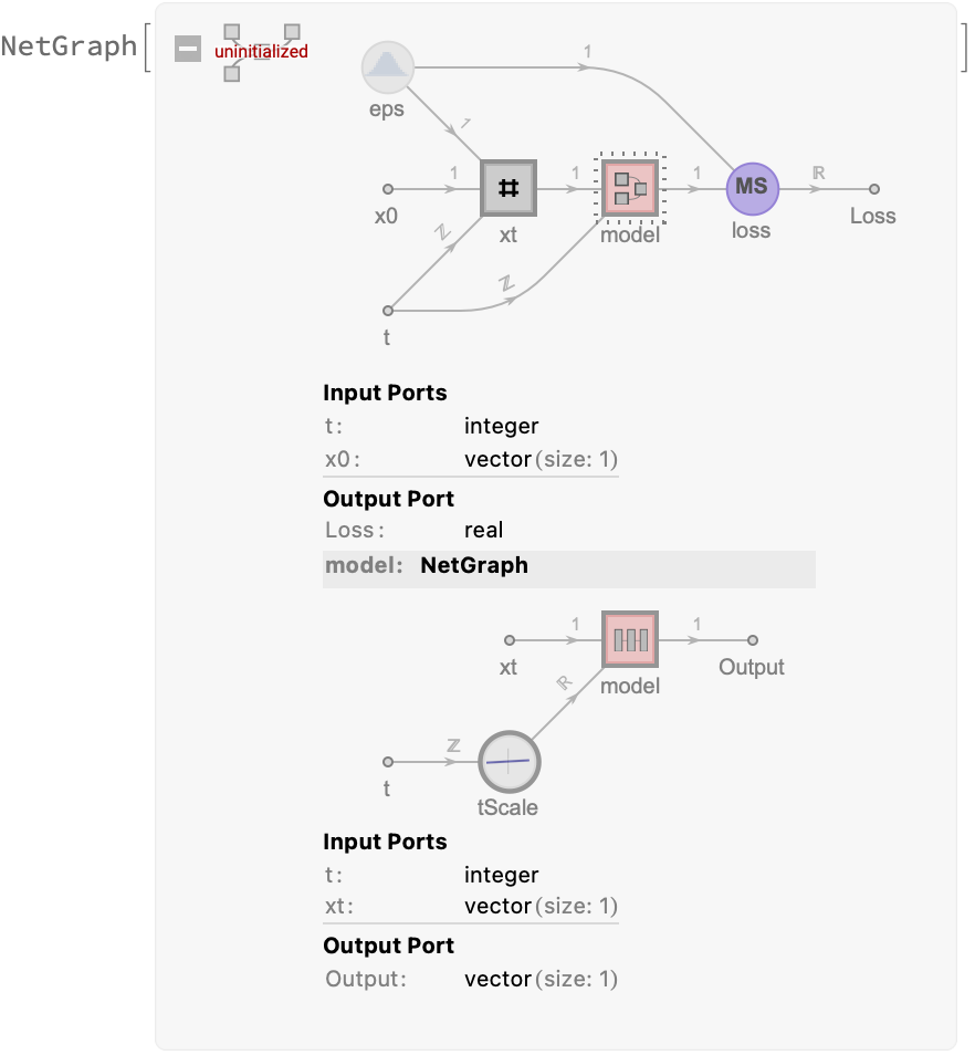
Having constructed the diffusion process, our next step is to develop a model that can undo the diffusion. It needs to take the time and the “diffused” x as inputs. We’ll rescale the time so that it is between -1/2 and +1/2, and just run this through a few fully-connected layers. There’s no rhyme or reason to this particular network architecture, and I’m sure it is totally overkill for the problem. After defining the model, we’ll use a NetGraph to put it together with the other pieces. We’ll need a set of parameters to define the model, so we’ll save those in an association for convenience.

(*convenience function for defining parameters*)
parameters[nDim_, tMax_, nH_] := <|"nDim" -> nDim, "tMax" -> tMax, "nHidden" -> nH|> 
  
 (*allow our xt to accept the parameter association*) 
  xt[param_Association] := xt[param["tMax"]] 
  
 (*define a network for generating random normal numbers*) 
  eps[param_Association] := With[{nDim = param["nDim"]}, 
    RandomArrayLayer[NormalDistribution, "Output" -> {nDim}]] 
  
 (*the "undiffusion" model that we will learn; appends a time *) 
  model[param_Association] := With[
    {tMax = param["tMax"], nDim = param["nDim"], nHidden = param["nHidden"]}, 
    NetGraph[
     <|"tScale" -> FunctionLayer[(# - 1)/(tMax - 1) - 0.5 &, Input -> "Integer"], 
      "model" -> NetChain[
        {AppendLayer["Input" -> nDim, "Element" -> "Real"], 
         LinearLayer[nHidden], Ramp, 
         LinearLayer[nHidden], Ramp, 
         LinearLayer[nHidden], Ramp, 
         LinearLayer[nDim]}]|>, 
     {NetPort["t"] -> "tScale", 
      {NetPort["xt"], "tScale"} -> "model"}]] 
  
 (*construct the network for learning the diffusion undoer*) 
  trainingNet[param_Association] := NetGraph[
    <|"eps" -> eps[param], 
     "xt" -> xt[param], 
     "model" -> model[param], 
     "loss" -> MeanSquaredLossLayer[]|>, 
    { {NetPort["t"], NetPort["x0"], "eps"} -> "xt", 
     {NetPort["t"], "xt"} -> "model", 
     {"model", "eps"} -> "loss"}, 
    "t" -> "Integer", "x0" -> {param["nDim"]}] 
  
 (*pull a sample for SGD*) 
  sampler[param_Association, trainingSample_List] := Function[ 
     <|"x0" -> RandomSample[trainingSample, #BatchSize], 
      "t" -> RandomInteger[param["tMax"], #BatchSize]|>];

Let’s try it on our 1D example. Let’s get a sense of the model architecture:

trainingNet@parameters[1, 200, 128]

Now let’s perform the calculation. Our training data consists of samples drawn from the training data and random times (using the sampler function defined above) to generate these data on demand (maybe there’s a more efficient way to do this by building a network that generates t and feeds it in, so we can just pass the entire collection of datapoints in?). Oh well.

How long should you train for? I’ve found that the loss function is not a great indicator of training quality (more on this below), so I’m just going to set a boundary of 2 minutes and stop there. The hyperparameters defining the network are also chosen pretty much at random; of course you can do better:

param = parameters[1, 200, 128]
trainedNet1D = NetTrain[trainingNet[param], sampler[param, trainingSample1D], 
   TimeGoal -> 120] (*train for 2 minutes on CPU*)

(*<|"nDim" -> 1, "tMax" -> 200, "nHidden" -> 128|>*)

Generating samples

Now we’ve got to extract the trained model and use it to generate new samples. We’ll start by defining the functions that let us do this. It is more natural to apply a Fold operation

  z[nSamples_, t_Integer] := RandomVariate[NormalDistribution[], nSamples] 
  z[nSamples_, 1] := ConstantArray[0., nSamples] 
   
   timeStep[alpha_List, alphaBar_List, sigma_List, trainedModel_NetGraph][x_, t_Integer] := With[
     {output = NetMapThreadOperator[trainedModel]@
        <|"xt" -> x, "t" -> ConstantArray[t, Length[x]]|>, 
      zVec = z[Dimensions[x], t]}, 
     1/Sqrt[alpha[[t]]]*(x - (1 - alpha[[t]])/Sqrt[1 - alphaBar[[t]]]*output) + sigma[[t]]*zVec 
    ] 
   
   generate[trainedNet_NetGraph, param_Association, nSamples_Integer] := 
    With[
     {trainedModel = NetExtract[trainedNet, "model"], 
      a = alpha@param["tMax"], 
      ab = alphaBar@param["tMax"], 
      sig = sigma@param["tMax"]}, 
     Fold[
      timeStep[a, ab, sig, trainedModel], 
      RandomVariate[NormalDistribution[], {nSamples, param["nDim"]}], (*x*)
      Reverse@Range[param["tMax"]] (*tValues*)]]

Now apply it to the model we trained above:

Histogram@Flatten@generate[trainedNet1D, param, 10^4]

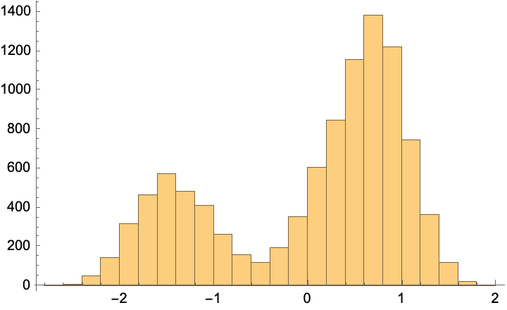
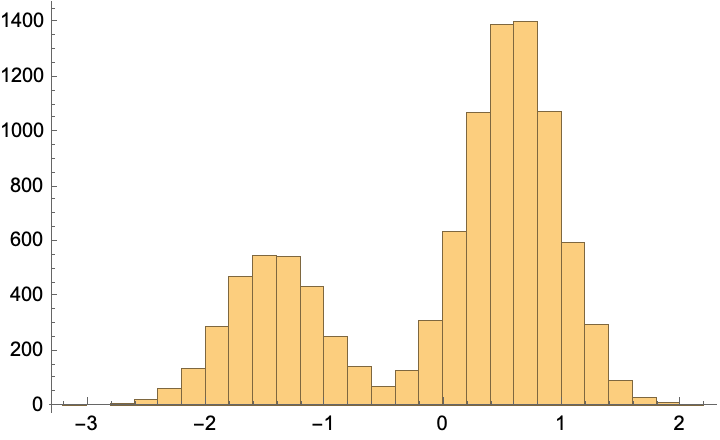
This almost exactly reproduces the training data (which we’ve seen before):

Histogram@Flatten@trainingSample1D

It’s also fun to compare to with Mathematica’s built in distribution learning methods–this defaults to performing a kernel density estimate:

With[
  {auto = LearnDistribution[Flatten[trainingSample1D]]}, 
  Histogram[RandomVariate[auto, 10^4], {0.1}, "PDF"]]

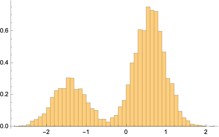
Our little diffusion model has done quite well for itself (of course, it is a bit of overkill for such a simple problem), but our goal is to illustrate the point.

Application to the 2D Problem

Let’s apply it to our spiral 2D problem. We’ll just use a humongous network with an arbitrarily chosen and almost certainly too large number of hidden layers, and see how well we do with 200 time steps:

param = parameters[2, 200, 256]
trainedNet = NetTrain[
   trainingNet[param], sampler[param, trainingSample2D], 
   Method -> "ADAM"]
Histogram3D@generate[%, param, 10^4]

(*<|"nDim" -> 2, "tMax" -> 200, "nHidden" -> 256|>*)

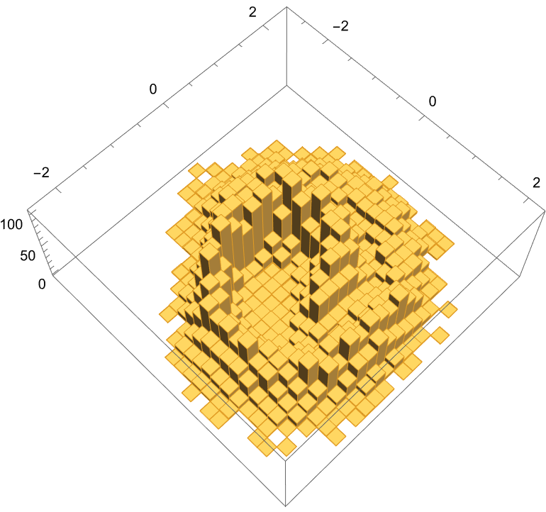
Not bad! We’re certainly capture some of the aspects of the spiral, it’s not as clean as we might like.

Let’s train the heck out of it (we’ll just start from where we left off. This will take ~6 minutes on CPU, provide you don’t overheat your poor laptop). Again, this is probably too much, but maybe it is useful. For each of our samples we have 200 times to consider, so maybe 10^5 training rounds is not too unreasonable.

trainedNetv2 = NetTrain[
    trainedNet, sampler[param, trainingSample2D], 
    Method -> "ADAM", MaxTrainingRounds -> 10^5] 
 
Histogram3D@generate[%, param, 10^4]

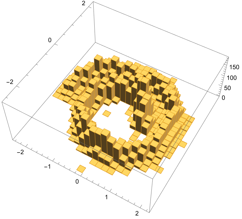
Perhaps it is easier to compare these as a DensityHistogram:

DensityHistogram /@ {trainingSample2D, 
    generate[trainedNet, param, 10^4], 
    generate[trainedNetv2, param, 10^4]} // GraphicsRow

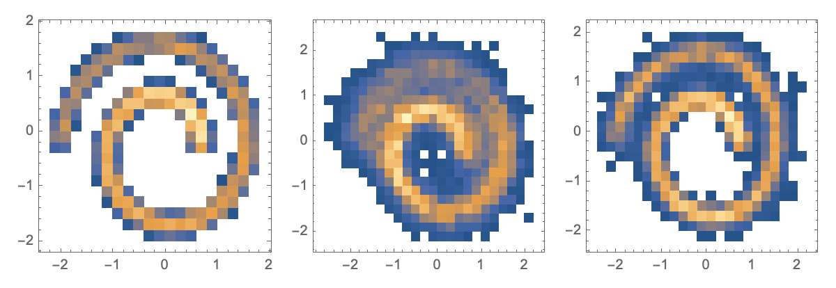
This suggests that you really do need to run long training rounds like 10^5. But now we see a good reproduction of the underlying probability distribution. Other parameters might include changing the number of time steps that are taken; using 1000 steps (instead of 200) might allow for finer resolution. This is left as an exercise for the reader…

From “Diffusion” to “Stable Diffusion”

So far we’ve implemented a “vanilla” diffusion model. The core idea behind stable diffusion is that one trains an autoencoder to generate the samples, and then performs diffusion in the latent space of the autoencoder. (In contrast, in the example above, we’re performing the diffusion process directly in the sample space).

You really need a larger example than this (like generating MNIST images) to show the value of this, but the MNIST autoencoder described in the Mathematica documentation would be a good starting point.

ToJekyll["Minimal diffusion model from scratch for generative machine learning", "ml machinelearning"]