Predicting Rare Earth Element Separation Chemistry

For a new project on f-element (rare earths and actinide) separation, I am trying to wrap my head around the literature. There is a very nice recent result from De-en Jiang and co. where they created a dataset of 1600 lanthanide rare-earth separation experiments, featurizing the extractant molecules with fingerprints and RDKit style features, featuring the solvents with some properties, and featurizing the metals themselves with a few periodic properties. (Liu et al, “Advancing Rare Earth Separations” JACS Au 2022 https://doi.org/10.1021/jacsau.2c00122 ). The supporting information contains the compete dataset (yay!) but not the neural network that they trained (although it describes it in the text). Let’s reproduce their result by training our own neural network…

Data Import and Preparation

Obtain data from supporting information; this is in the form of an excel spreadsheet, so download it to the local directory and pull it in. The training and test set are conveniently in separate sheets. We will need to drop the last column (which is a literature reference) and then format it appropriately, so we write a simple function (prepareData) to facilitate this:

SetDirectory@NotebookDirectory[]; 
  
 (*save a copy of the feature names for later reference*)
{featureNames, tr} = TakeDrop[#, 1] &@ Import["au2c00122_si_002.xlsx", {"Data", "training set"}]; 
  
 (*drop the last column which indicates the reference and use the second-to-last column as the output value*) 
prepareData[data_?MatrixQ] := ResourceFunction["TableToTrainingSet"][data[[All, ;; -2]], -1] 
 
trainingSet = prepareData[tr]; 
  
 (*used to check the results after training*)
validationSet = prepareData@Rest@Import["au2c00122_si_002.xlsx", {"Data", "validation set"}];

And a quick sanity check to make sure they are distinct:

ContainsAny[validationSet, trainingSet] (*inputs and outputs identical?*)
ContainsAny[validationSet[[All, 1]], trainingSet[[All, 1]]] (*inputs are the same?*)


(*False*)

(*False*)

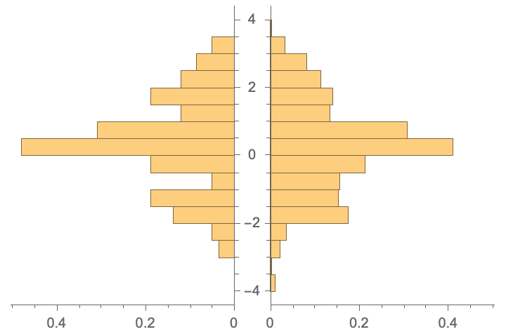
Probability distribution of outputs is similar (as these were extracted from the same studies:):

PairedHistogram[
  validationSet[[All, 2]], trainingSet[[All, 2]], 
  Automatic, "PDF"]

Model Construction

Goal: Reproduce the optimal neural network model in their study (a plain vanilla feed-forward network, the only wrinkle being that they use a PreLU aka ParametricRampLayer).

Comment: It seems unusual to me that they do not use DropoutLayers and/or BatchNormalizationLayer to deal with the problem of overfitting. Perhaps this is something to investigate in the future; for now we will just reproduce what they did, using the optimal hyperparameters they report. They use stochastic gradient descent, so we will too.

(*extracted from Table S1*)
  hyperparameter = <|"weight decay" -> 0.01, "learning rate" -> 0.00001, "epochs" -> 15000|>; 
   
  (*define general architecture*) 
  (*we don't strictly need to provide the input size in this definition, as NetTrain can figure it out later, but doing so now lets us count parameters*) 
   net = NetChain[
     {LinearLayer[512], ParametricRampLayer[], 
      LinearLayer[128], ParametricRampLayer[], 
      LinearLayer[16], ParametricRampLayer[] , 
      LinearLayer[{}] }(*scalar output*), 
     "Input" -> Length@First@First@trainingSet ] 
   
  (*query the network to find out about parameters, etc.*) 
   Information[net]

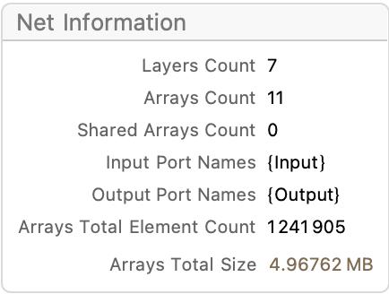
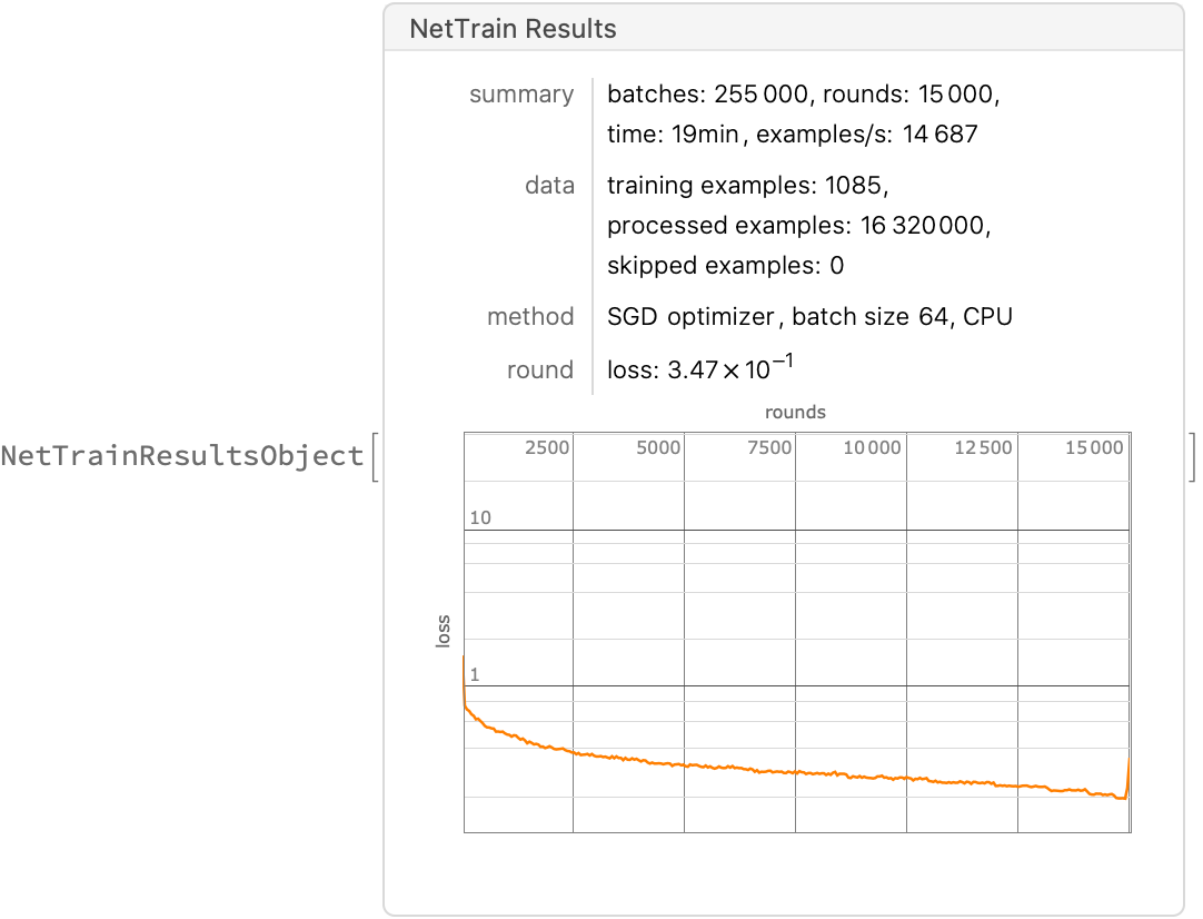
Now proceed to train the network (this takes about 15-20 minutes, running on CPU on my laptop). Specifying the third parameter All returns a NetTrainResultsObject describing the process; excluding this will just returned the trained network (which is fine, but maybe we want to know aspects of how the model got trained).

If I needed to do something more ambitious, I would think about using the RemoteBatchSubmit functionality to do the training (as the dataset is small and could just be sent up to a remote server). I took this as an opportunity to write the explanatory text in this notebook and make a coffee :-)

Comment: In the paper they state: In each epoch, 80% of the 1085 data points were randomly selected for training. I originally thought that this would be done by the ValidationSet option below, but that chooses only a fixed set of parameters. I am not actually sure how to do this randomly at each epoch, so will just going to skip having a validation set term for now, but I asked about it on StackOverflow). Give how little data we have it is worth making sure it all gets in (the metrics computed at the end are indeed lower without them), so we’ll just comment out the ValidationSet setting for now.

result = NetTrain[net, trainingSet, All, 
   LossFunction -> MeanAbsoluteLossLayer[],(*aka L1 loss*)
  (*ValidationSet->Scaled[0.2],*) 
   LearningRate -> hyperparameter["learning rate"], 
   Method -> {"SGD", "L2Regularization" -> hyperparameter["weight decay"]} , 
   MaxTrainingRounds -> hyperparameter["epochs"]]

Save the results for a rainy day (and extract the trained network for further use):

Save["result.wl",result]; (* complete net results object on training history*)
trainedNet = result["TrainedNet"]
Export["trainedNet.wlnet", trainedNet] (*just the trained weights*)

(*"trainedNet.wlnet"*)

Model evaluation

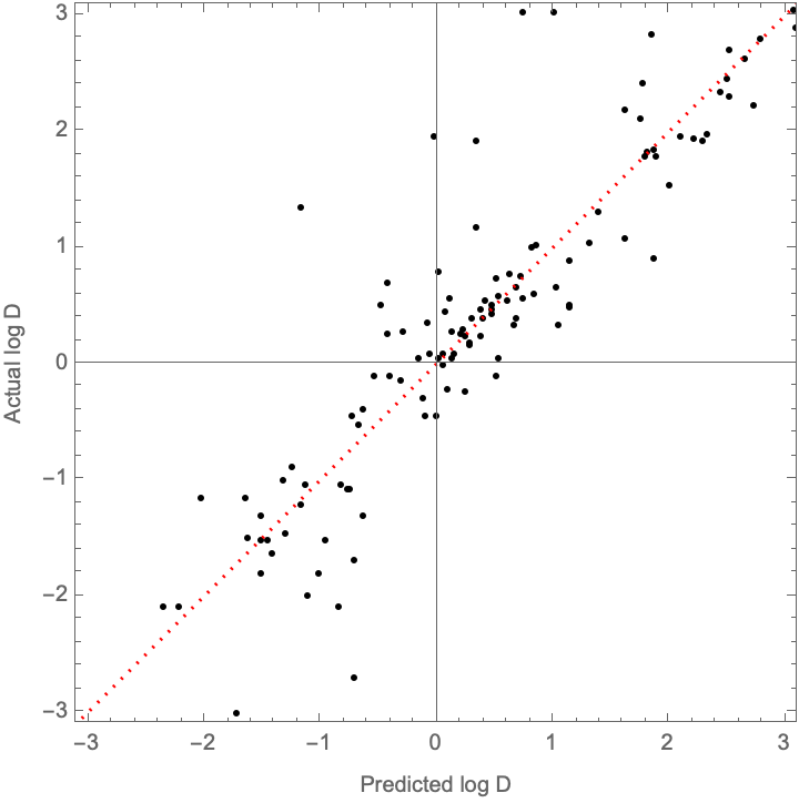
How well does the model reproduce the training data and the validation data? MeanDeviation corresponds to MAE and StandardDeviation corresponds to RMSE:

NetMeasurements[trainedNet, trainingSet, {"RSquared", "MeanDeviation","StandardDeviation"}]

(*{0.909177, 0.190673, 0.412244}*)

NetMeasurements[trainedNet, validationSet, {"RSquared", "MeanDeviation", "StandardDeviation"}]

(*{0.78438, 0.406454, 0.633028}*)

This is a bit worse than what is reported in the supporting information (validation data of R^2 = 0.85, MAE = 0.34, and RMSE = 0.53), but we’re clearly on the right track here. How do the values compare?

With[
  {predictedD = trainedNet /@ validationSet[[All, 1]], 
   actualD = validationSet[[All, 2]], 
   parityLine = Plot[x, {x, -4, 4}, PlotStyle -> { {Red, Dotted}}] 
  }, 
  Show[
   ListPlot[
    Transpose[{predictedD, actualD}], 
    Frame -> True, FrameLabel -> {"Predicted log D", "Actual log D"}, 
    AspectRatio -> 1, PlotRange -> { {-3.1, 3.1}, {-3.1, 3.1}}, PlotStyle -> Black], 
   parityLine]]

How well does this perform relative to a Random Forest/GBT models?

Comment: A limitation in the paper is that they don’t have a baseline. So let’s make one with a simple random forest and GBT models. For reference, the random forest trains in about 5 seconds and the GBT in about 30 seconds:

rf = Predict[trainingSet, Method -> "RandomForest", PerformanceGoal -> "Quality"]
PredictorMeasurements[%, validationSet]
%[{"RSquared", "MeanDeviation", "StandardDeviation"}]

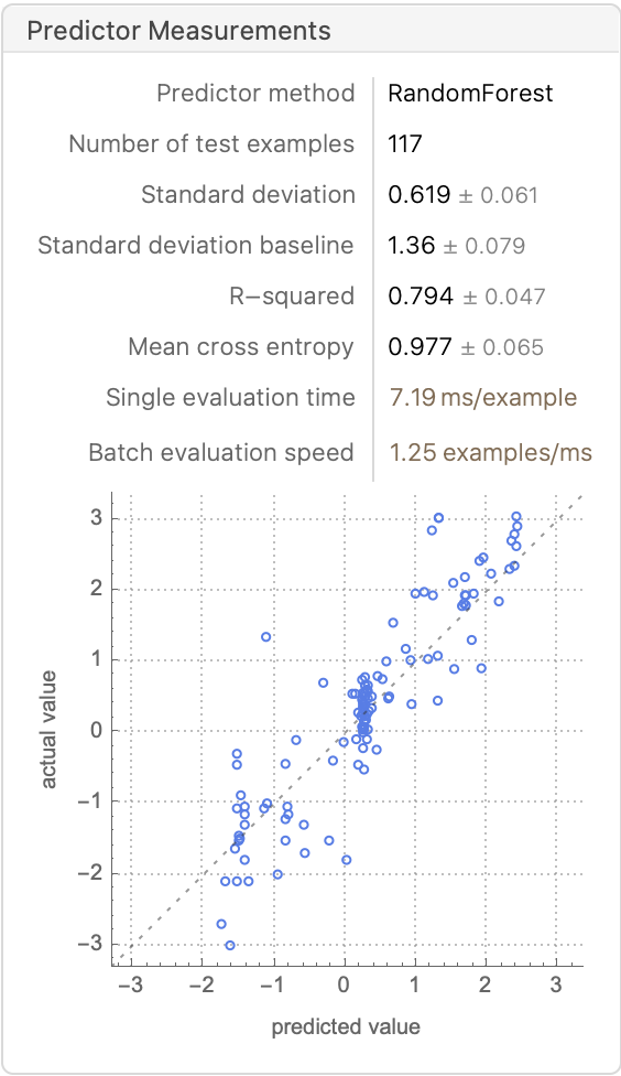
(*{0.794043, 0.440639, 0.618681}*)

gbt = Predict[trainingSet, Method -> "GradientBoostedTrees", PerformanceGoal -> "Quality"]
PredictorMeasurements[%, validationSet]
%[{"RSquared", "MeanDeviation", "StandardDeviation"}]

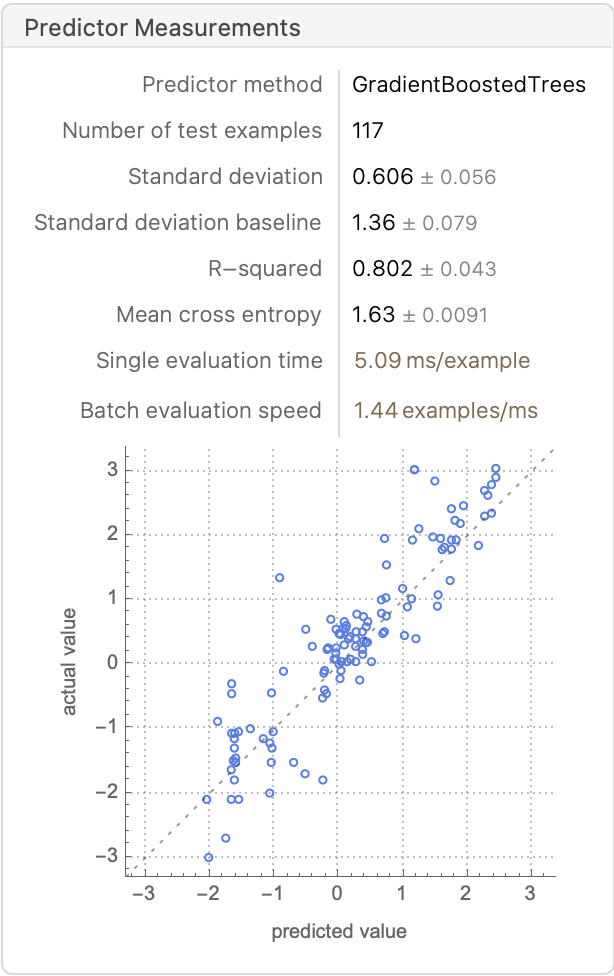
(*{0.802496, 0.442316, 0.605852}*)

Comparing these results to the ones from our neural network fit {0.78438, 0.406454, 0.633028} and the paper’s reported results {0.85, 0.34, 0.53}, we can see that a simple RF or GBT without extensive hyperparameter tuning essentially reproduces the best results in the paper, with only a fraction of the compute resources. This might open the door for doing a conformal prediction using the cheaper RF model. Johansen et al. discuss specific implementation details about regression conformal prediction with RF

Addendum: Optimizing using ADAM (27 Feb 2023)

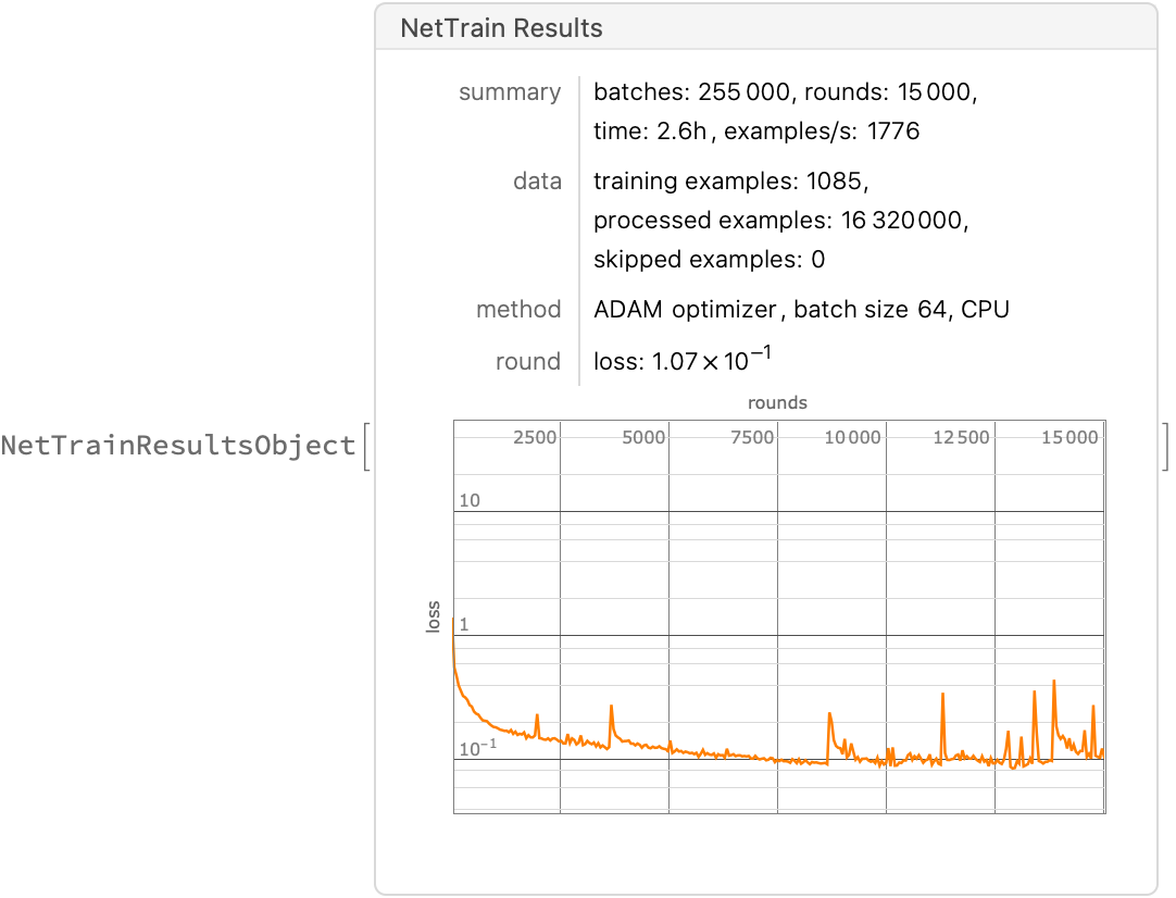
What if we try using default learning parameters (ADAM as an optimizer, etc.)? Let’s retrain and find out:

result2 = NetTrain[net, trainingSet, All, 
   LossFunction -> MeanAbsoluteLossLayer[],(*aka L1 loss*)
   MaxTrainingRounds -> hyperparameter["epochs"]]

Save["adamNet.wl", result2]; (* complete net results object on training history*)
adamNet = result2["TrainedNet"]
Export["adamNet.wlnet", adamNet] (*just the trained weights*)

(*"adamNet.wlnet"*)

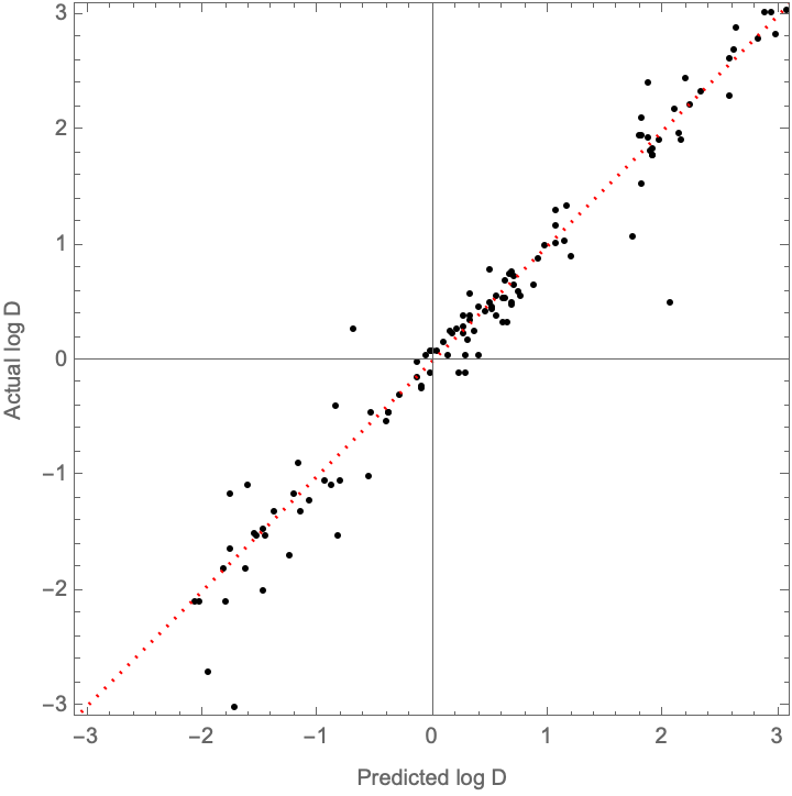
How well does it compare to the results in the paper (recall that they report report: {0.85, 0.34, 0.53})?

NetMeasurements[adamNet, #, {"RSquared", "MeanDeviation", "StandardDeviation"}] & /@ {trainingSet, validationSet}

(*{ {0.99287, 0.0618658, 0.115507}, {0.950707, 0.188798, 0.30267}}*)

Awesome! We beating their metrics (although again, I suspect there may be some backdoor overfitting)

With[
  {predictedD = adamNet /@ validationSet[[All, 1]], 
   actualD = validationSet[[All, 2]], 
   parityLine = Plot[x, {x, -4, 4}, PlotStyle -> ] 
  }, 
  Show[
   ListPlot[
    Transpose[{predictedD, actualD}], 
    Frame -> True, FrameLabel -> {"Predicted log D", "Actual log D"}, 
    AspectRatio -> 1, PlotRange -> { {-3.1, 3.1}, {-3.1, 3.1}}, PlotStyle -> Black], 
   parityLine]]

Next Steps/Improvements

• Can we further improve the fit?

• Try using Dropout/BatchNorm to limit overfitting?

• Apply this model to our own experimental data for lanthanides

• Expand the datasets to actinides

• Implement custom featurizers

NotebookFileName[]
ToJekyll["Predicting Rare Earth Element Separation Chemistry", "science, machinelearning, ml"]

(*"/Users/jschrier/Dropbox/journals/science/2023.02.25_jiang_lanthanide_model/2023.02.25_jiang_lanthanide_model.nb"*)