Conformal prediction example

Conformal prediction computes confidence intervals associated to any black box prediction method, without assuming any prior model on the sample in the dataset. More formally, conformal prediction bounds the miscoverage: P(Y notin set)<=α by computing the interval as quantile of runs of the method over the points in the dataset. I was inspired to think through this Gabriel Peyré’s post, and the notes below closely follow his notebook…

Addendum (01 July 2023): A nice youtube video explaining full conformal predictors

We begin by defining some example data, defined as a cubic polynomial, and adding random noise. We will then try to learn the function based on the noisy samples, but I will plot the exact samples as well to give us a sense of how well our fit performs (even though in practice we don’t have access to this type of data):

phi0[x_] := {x*0 + 1, x, x^2, x^3} (*the function*)
nPoints = 200; (*how many sample points*)
x0 = RandomReal[{-3.5, 4.5}, nPoints]; (*inputs*)
w0 = {0, -5, 0, 1} ;(*exact ("unknown") coefficients for the function*)
y0 = w0 . phi0[x0] + RandomVariate[NormalDistribution[], nPoints]*7; (*noisy samples*)
yExact = w0 . phi0[x0]; (*exact values...not known to the learner*)
 
 data = ListPlot[
   {Transpose[{x0, y0}], Transpose[{x0, yExact}]}, 
   PlotStyle -> {Gray, Green}, PlotLegends -> {"Noisy data", "Exact"}]

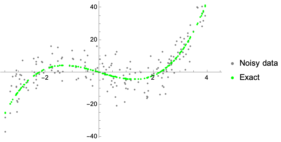
In general, conformal prediction works for any black-box method. For illustration purposes, we’ll consider a simple least-squares estimator, solving the function by taking the pseudoinverse. The data is stored in X = (xi) and Y = (yi) , with w being the learned weights. So far, this is just good-old fashioned least-squares fitting:

phi[x_] := {x*0 + 1, x, x^2, x^3} (*general functional form to learn*) 
 
hatW[x_, y_] := y . PseudoInverse[phi[x]] (*determine weights in function*)
hatY[x_, w_] := w . phi[x] (*make a prediction for Y, given the learned weights*) 
 
predictions = ListPlot[
    Transpose[{x0, hatY[x0, hatW[x0, y0]]}], 
    PlotStyle -> Red, PlotLegends -> {"Fitted"}];
Show[data, predictions]

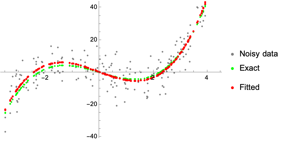
The conformance function S(x,y|X,Y) checks the accuracy of the prediction–a common choice is merely the absolute difference between the prediction and the observed values. We implement it as a function of the learned weights:

conformanceS[x_, y_, w_] := Abs[y - hatY[x, w]]
conformancePlot = ListPlot[
    Transpose[{x0, conformanceS[x0, y0, hatW[x0, y0]]}], 
    PlotStyle -> Blue];
Show[data, predictions, conformancePlot]

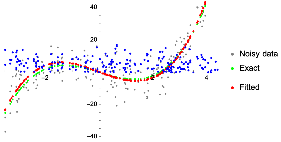
Given a conformance function, S, the conformal prediction gives a score by computing the rank of conformance at the point of interest among all possible scores at the samples. Think about this in the following way: Suppose we add some new point (x,y) to the training data and retrain the model, obtaining some new optimized parameters w. With these optimized parameters, we can ask the rank that this new point would have relative to the existing points. An extreme rank would suggest it is quite unlikely. In practice this defines an interval around the predictions.

conformal[x0_, y0_][x_, y_] := With[
   {w = hatW[Append[x0, x], Append[y0, y]], (*new fitted weights with new datapoint*)
    nPoints = Length[x0]}, 
   With[
    {v = MapThread[ conformanceS[#1, #2, w] &, {x0, y0}], (*conformance of old points*)
     vPoint = conformanceS[x, y, w]}, (*conformance of the new point*)
    (1 + Total@Boole@Map[LessEqualThan[vPoint], x0])/(nPoints + 1)(*what's the point rank?*) 
   ] ]

For example, suppose that we set x = 0, and ask what ranges of y we might expect our function to have given the data.

Plot[conformal[x0, y0][0, y], {y, -10, 10}]

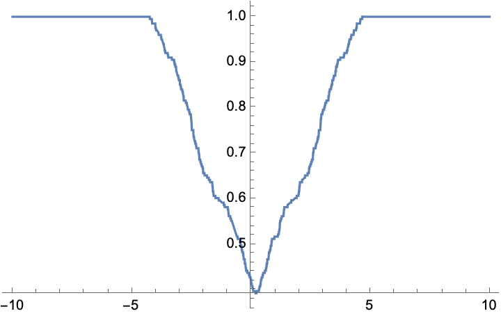
What values of y that are within the 95% interval?

Minimize[ {Abs[conformal[x0, y0][0, y] - 0.95], y < 0}, y]
Minimize[ {Abs[conformal[x0, y0][0, y] - 0.95], y > 0}, y]

(*{0.000248756, {y -> -3.7298}}*)

(*{0.000248756, {y -> 4.15204}}*)

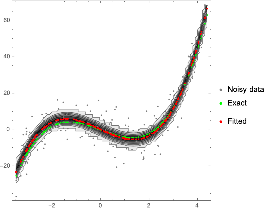
Go ahead and compute a grid of values, plotting the confidence intervals as the level set (contour plot) of the conformance function:

nx = 80;
ny = 70;
xList = Subdivide[Min[x0], Max[x0], nx];
yList = Subdivide[Min[y0], Max[y0], ny];
conformanceGrid = Table[conformal[x0, y0][ix, iy], {iy, yList}, {ix, xList}];

contour = ListContourPlot[conformanceGrid, 
    DataRange -> {MinMax[xList], MinMax[yList]}, ColorFunction -> GrayLevel];
Show[contour, data, predictions]

NotebookFileName[]
ToJekyll["Conformal prediction example", "machinelearning"]

(*"/Users/jschrier/Dropbox/journals/mathematica/2022.07.05_conformal_prediction_implementation.nb"*)