Eliciting priors from LLMs by Gibbs Sampling

In a recent pre-print, Zhu and Griffith describe a method for Eliciting the Priors of Large Language Models using Iterated In-Context Learning. The core idea is to adapt a procedure used to perform Markov Chain Monte Carlo with People. Effectively, this implements a Gibbs sampler for the joint distribution p(d, h) = p(d|h)p(h), and the stationary distribution on hypotheses is the prior p(h). Samples from the prior are obtained by running the iterated learning process long enough to converge to the distribution. Let’s replicate their result and compare to direct sampling…

Background

They depict their method schematically as follows:

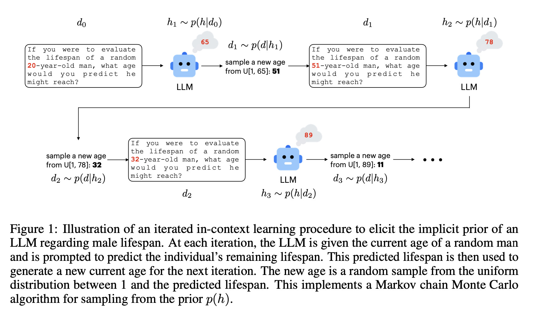
The authors describe their method as:

To test the hypothesis that iterated in-context learning should reveal the prior distributions of LLMs, we incorporated GPT-4 into a prompt-based iterated learning procedure. At each iteration t, GPT-4 undertakes a prediction task using the data d_{t-1}. The model’s prediction is recorded as ht. Subsequently, we employ generic likelihood functions that are a reasonable match for the sampling process producing the described data to randomly generate the data for the next iteration, dt ~ p(d|ht). For instance, we applied the method depicted in Figure 1 to investigate GPT-4’s prior beliefs about men’s lifespans. In this procedure, the LLM is prompted to estimate the lifespan of a random man, given information about his current age. The age of the man encountered in the next prompt is then uniformly sampled from a range extending from 1 to the lifespan predicted in the previous iteration, matching the probability of randomly encountering the man at this point in his life. By iteratively applying this procedure, we expect the final prediction made by GPT-4 will converge on a stationary distribution that reflects the model’s prior beliefs about human life expectancy.

In the experiments presented in the remainder of the paper, 100 iterated learning chains were implemented with random seeds. We conducted 12 iterations for each chain. The temperature of GPT-4 was fixed at 1, consistent with the idea of sampling from the posterior.

Implementation

The life expectancy example seems a bit morbid, so for more whimsy, we will use their cake-baking example, using the prompt text from Appendix A . The general strategy is to define an LLMFunction that performs the iteration, and then a sampling function that generates the next iteration in the chain:

Clear[query, sample, result] 
  
 (* define the query *)
query[model_] := LLMFunction[
    "Imagine you are in somebody's kitchen and notice that a cake is in the oven. The timer shows that it has been baking for `` minutes. How long do you expect the total amount of time to be that the cake needs to bake? Please provide your prediction as a single number. Do not include any additional text or explanation in your response.", 
    Integer,(*output format*)
    LLMEvaluator -> 
     <|"Model" -> model, 
      "Temperature" -> 1, 
      "Prompt" -> "You are an expert at predicting future events." |>,
    ProgressReporting -> False]  
  
 (* define the sampling procedure *)
sample[q_][dPrev_Integer] := q@ RandomInteger[dPrev]

What does the progression of one chain look like?

result = Rest@ NestList[sample[query["gpt-4o-2024-05-13"]], 120, 12]

(*{80, 75, 60, 45, 30, 40, 30, 30, 45, 60, 30, 45}*)

Assuming that 12 trials is enough to converge to the stationary distribution, we need only the last item, so we will use Nest and obtain 100 chains in parallel:

result2 = ParallelTable[
    Nest[sample[query["gpt-4o-2024-05-13"]], 120, 12], (* chain function *)
    100]; 

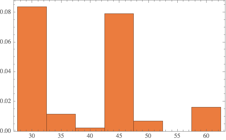
Now visualize the underlying distribution of priors–it makes sense that we would expect the times to be 30, 45, or 60 minutes as common baking times. (There is of course no good reason that these are optimal for a cake, but these types of patterns in reaction conditions are similar to my previous observations about anthropogenic dataset biases in chemical procedures.)

Histogram[result2, Automatic, "PDF"]

As an aside, there are occasionally errors in which the model does not return an integer; these get suppressed in our result depicted above:

CountsBy[IntegerQ]@ result2

(*<|True -> 86, False -> 14|>*)

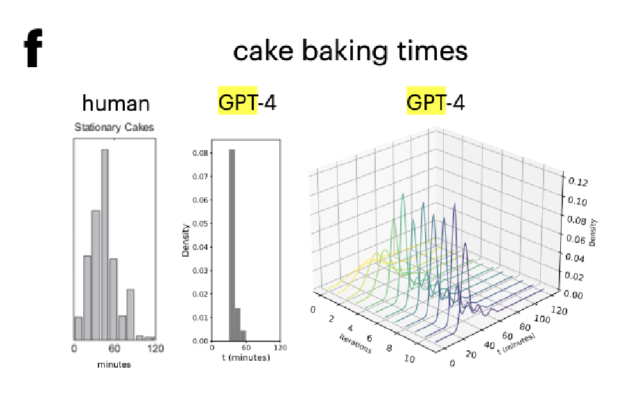
Interestingly, the resulting distribution appears different from Figure 5f, which appears to have only a single common peak at 30 minutes:

Comparison to GPT-4-turbo

The authors say they use GPT-4 without specifying a particular model. So maybe we should see how this compares to our old workhorse, GPT-4-turbo?

result2b = ParallelTable[
     Nest[sample[query["gpt-4-0125-preview"]], 120, 12], (* chain function *)
     100]; 
 
Histogram[%, Automatic, "PDF"]

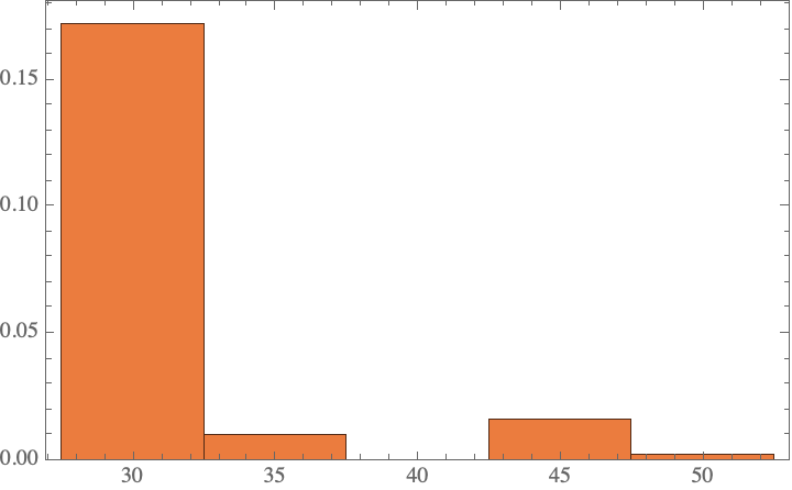
This seems more consistent with their results.

Additionally, GPT-4-turbo is much better at complying with the instructions:

CountsBy[IntegerQ]@ result2b

(*<|True -> 100|>*)

(As a side note, I found that GPT-3.5-turbo was relatively unreliable at following the instructions to return only the integer value, so it breaks:)

result2c = ParallelTable[
     Nest[sample[query["gpt-3.5-turbo-0125"]], 120, 12], (* chain function *)
     100]; 
 
Histogram[%, Automatic, "PDF"]
CountsBy[IntegerQ]@%%

(*<|False -> 100|>*)

Comparison to Direct Sampling

Why not just perform direct sampling approach? The authors did not do this… I will take the conservative strategy of rewriting their prompt, deleting the prior information and mostly keeping everything else the same (except to specify that the total time should be in minutes):

query2[model_] := LLMFunction[
   "Imagine you are in somebody's kitchen and notice that a cake is in the oven. How long do you expect the total amount of time (in minutes) to be that the cake needs to bake? Please provide your prediction as a single number. Do not include any additional text or explanation in your response.", 
   Integer,(*output format*)
   LLMEvaluator -> 
    <|"Model" -> model, 
     "Temperature" -> 1, 
     "Prompt" -> "You are an expert at predicting future events." |>, 
   ProgressReporting -> False] 

Now, instead of a chain, we just make a single query to get the prediction:

query2["gpt-4o-2024-05-13"][]

(*35*)

Repeat this to obtain 100 predictions, using GPT-4o, because it is cheaper and faster. The resulting distribution is quite different from the Gibbs sampling approach obtained above:

result3 = ParallelTable[
    (query2["gpt-4o-2024-05-13"][]), 
    100];
Histogram[%, Automatic, "PDF"]

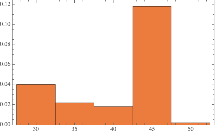
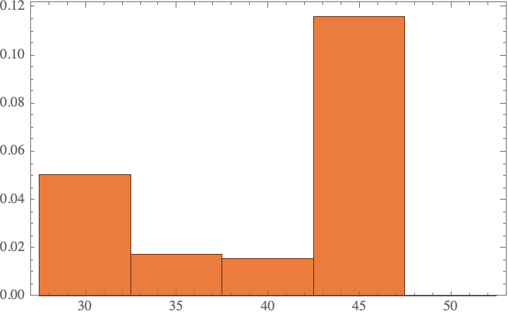
Now one might quibble that we have only done 100 evaluations, whereas the Gibbs sampling approach performed 1200 evaluations. Maybe we are just not sampling enough to see a good distribution? What if we make the same number of function calls? It turns out that the result is effectively same as the 100 sample case, so this does not make a difference:

result4 = ParallelTable[
     (query2["gpt-4o-2024-05-13"][]), 
     12*100]; 
 
Histogram[%, Automatic, "PDF"]

Conclusions

• In addition to predicting quantities (as done above), they also demonstrate applications to causal learning and proportion estimation. It may be fun to apply this to problems we care about.

• It is surprising that the prior distributions differ so much between GPT-4o and GPT-4-turbo.

• Future work:

  • Apply to the German Tank problem?

ToJekyll["Eliciting priors from LLMs by Gibbs Sampling", "llm statistics gpt4"]