Semisupervised Twin Regression

Pairwise difference regression (aka twin regression) is an underappreciated meta-ML approach. The idea is to to take pairs of inputs (x1, x2) and train your model to predict y1-y2. One advantage is that this gives you N^2 training points (handy for those small-data science problems). At inference time, you select a sample of known reference x->y data, and generate an estimate of the distribution of pairwise distances from those references for the point of interest. Thus, the second advantage is that you get an approximate form of uncertainty quantification without having to train multiple models. Wetzel et al described this using neural networks (which they denote as twin neural networks) in 10.1002/ail2.78. Tynes et al describe a similar strategy using tree methods in 10.1021/acs.jcim.1c00670. But going beyond this, Wetzel et al. also describe a semisupervised version which trains on triples (doi:10.1088/2632-2153/ac9885) –the supervised examples have the typical MSE loss and the unspervised examples are evaluated for their internal consistency of the predictions (they should sum to zero). This gives you more data to train on and effectively regularizes the network for transductive (try to predict the labels of the unsupervised examples seen in training) or inductive (predict labels of examples that have not been seen at all), giving better performance. A minimal working implementation and demonstration of the idea…

General setup: Model Architecture and Sample Data

To be clear, this is not intended as a step-by-step reproduction of their work. In fact, I did not even use their code as a reference, I just thought through it based on the paper. And I do not mimic their specific training examples.

Comment: Reference 24 in their paper alleges to point to the source code, but it is to the wrong repository (!) The correct repository with their tensorflow implementation is [https://github.com/sjwetzel/PublicSemiSupervisedTNNR]

First, some general housekeeping. For demonstration we will use the same network to evaluate the supervised TNN and the semi-supervised (transductive) approach–a vanilla 2-layer model and the Wine Quality dataset. We will take only 1/3 of the data as labeled for training, standardizing the input values (Wetzel at all map this to [-1, +1] instead, but it accomplishes the same general idea):

(* define the underlying tnn*)
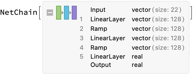
  tnn = NetChain[
      {LinearLayer[128], Ramp, 
       LinearLayer[128], Ramp, 
       LinearLayer[{}]}, 
      "Input" -> 22]; (*ordinarily we could infer input size, but not with a data generator*) 
   
  (*define the labeled and unlabeled dataset split*) 
   {labeled, unlabeled} = With[
      {d = ExampleData[{"MachineLearning", "WineQuality"}, "TrainingData"]}, 
      With[
       {scaledX = Standardize@d[[All, 1]], 
        y = d[[All, 2]]}, 
       TakeDrop[
        Thread[scaledX -> y], 
        UpTo@Round[Length[d]/3]]]];

Supervised Learning (Baseline Twin Regressor)

We will start by implementing the simple supervised twin neural network regressor.

Train the Model

Our main need is to generate inputs on demand by pairs of inputs and differences of outputs:

pairGenerator[d_][settings_] := With[
   {randomPairs = Table[RandomSample[d, 2], {settings["BatchSize"]}]},
   <|"Input" -> #[[1, 1]]~Join~#[[2, 1]], "Output" -> #[[1, 2]] - #[[2, 2]]|> & /@ randomPairs 
  ]

Now we can train the model using this data generator. Unless we specify the RoundLength option, the generator will only be called once per round; we want it to see all of the data, so we need to manually expand that. Wetzel et al use adadelta, learning rate decay and early stopping–for simplicity, I will just use the default Adam optimizer and forget it:

trainedPairTNN = NetTrain[
   tnn, 
   {pairGenerator[labeled], "RoundLength" -> Length[labeled]}, 
   LossFunction -> MeanSquaredLossLayer[], (*default, but say it anyway*)
   "MaxTrainingRounds" -> 2000]

Make a prediction

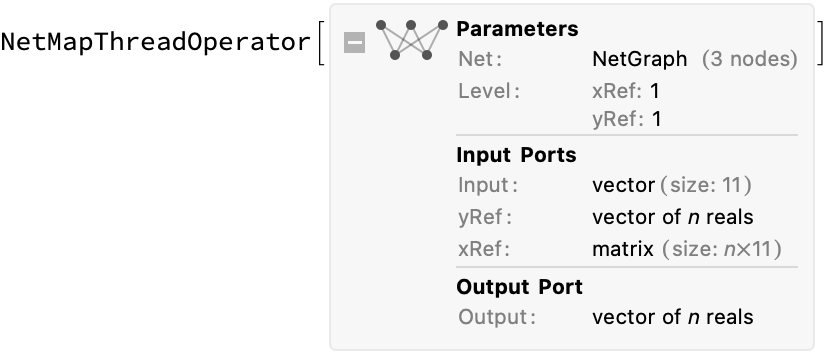
Now make a prediction of the output. We begin by defining a (neural network) function to compute the difference given a single reference value, then use NetMapThreadOperator to create a new neural network that maps it over an arbitrary length list of input reference x and y values. It is then useful to define a convenience function for making predictions with that network (just mapping to the proper inputs names):

prepareNetwork[tnn_, n_ : 11] := With[
    {single = NetGraph[
       {CatenateLayer[], tnn, FunctionLayer[#y2y1 + #yRef &]}, 
       {NetPort["Input"] -> 1 -> 2 -> 3, 
        NetPort["xRef"] -> 1}, 
       "xRef" -> n, 
       "Input" -> n, 
       "yRef" -> "Real"]}, 
    NetMapThreadOperator[single, <|"xRef" -> 1, "yRef" -> 1|>]] 
 
predict[net_, input_, ref_] := net[<|"Input" -> input, "xRef" -> ref[[All, 1]], "yRef" -> ref[[All, 2]]|>]

Apply it on a sample data point:

pairTNNRegressor = prepareNetwork[trainedPairTNN]
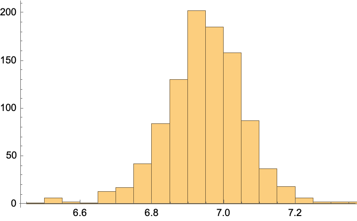
predictions = predict[%, unlabeled[[1, 1]], RandomSample[labeled, 1000]];
Histogram[%]
MeanAround[%%] (*mean and standard error*)
unlabeled[[1]] (*true value*)

(*{-0.223916, -0.947164, 0.203167, -0.945561, -0.851039, 0.0911935, -1.10973, -0.761609, 0.668289, -0.341423, 0.31335} -> 6.*)

Comment: We are off by about 1 (predict 6.9, true value is 6), but it is neat that we get an error estimate…

Semi-Supervised Model

Now we will implement the semi-supervised version. The main things we have to are implement the loss function and data generator; otherwise we can reuse much of the code defined above.

Train the model

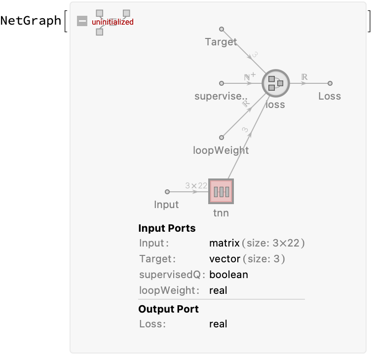
This requires a bit more work to set up the loss function to handle the mean square error and loop consistency losses. My general idea here was to have the training data include an indicator variable supervisedQ which tells the loss function which loss type to use; the loopWeight hyperparameter is also provided in this way.¹ NetMapOperator is used to perform weight sharing on the three identical pair regressors described in the paper:

(*define the loss function, with inputs that control whether to evaluate supervised or unsupervised versions*)
  loss = NetGraph[
      <|"mse" -> MeanSquaredLossLayer[], (*supervised Loss*)
       "loop" -> FunctionLayer[Total[#]^2 &],(*unsupervisedLoss*)
       "loss" -> FunctionLayer[#supervisedQ*#mse + #loopWeight (1 - #supervisedQ) #loop &] |>, 
      {NetPort["Input"] -> "mse", 
       NetPort["Target"] -> "mse" -> NetPort["loss", "mse"], 
       NetPort["Input"] -> "loop" -> NetPort["loss", "loop"], 
       "loss" -> NetPort["Loss"]} 
     ]; 
   
  (*define training architecture of the tnn*) 
   semisupervisedTNN = 
    NetGraph[
     <|"tnn" -> NetMapOperator[tnn], 
      "loss" -> loss|>, 
     {NetPort["Input"] -> "tnn" -> "loss"}, 
     "supervisedQ" -> Restricted["Integer", {0, 1}], 
     "loopWeight" -> "Real", 
     "Input" -> {3, 22}] (*must explicitly set input size to use a data generator*) 
  

Next define the process by which we generate data. Wetzel et al. provide half of the batch as supervised data and half as unsupervised data (which contains a mixed of supervised and unsupervised points). As defensive programming, I separate the unsupervised and supervised program paths to avoid accidentally leaking the labels. In short, this is really just written for clarity and quick hackery, rather than for speed in a production setting–it may be beneficial to compile this code to improve the speed.

subdivide[n_Integer] := With[
     { half = Round[n/2], 
       sixth = Round[n/6]}, 
    {half, sixth, sixth, n - half - sixth - sixth}] 
 
supervised[d_, hyperparam_] := 
   <|"Input" -> {d[[1, 1]]~Join~d[[2, 1]], d[[2, 1]]~Join~d[[3, 1]], d[[3, 1]]~Join~d[[1, 1]]}, 
    "Target" -> {d[[1, 2]] - d[[2, 2]], d[[2, 2]] - d[[3, 2]], d[[3, 2]] - d[[1, 2]]}, 
    "supervisedQ" -> 1, 
    "loopWeight" -> hyperparam|> 
 
unsupervised[d_, hyperparam_] := 
   <|"Input" -> {d[[1, 1]]~Join~d[[2, 1]], d[[2, 1]]~Join~d[[3, 1]], d[[3, 1]]~Join~d[[1, 1]]}, 
    "Target" -> {0, 0, 0}, 
    "supervisedQ" -> 0, 
    "loopWeight" -> hyperparam|> 
  
 (*purely supervised*)
sampleS[labeled_, _] := RandomSample[labeled, 3] 
  
 (*two labeled points, one unsupervised*)
sampleA[labeled_, unlabeled_] := RandomSample[
    RandomSample[labeled, 2]~Join~RandomSample[unlabeled, 1]] 
  
 (*one labeled, two unsupervised*)
sampleB[labeled_, unlabeled_] := RandomSample[
    RandomSample[labeled, 1]~Join~RandomSample[unlabeled, 2]] 
  
 (*purely unsupervised*)
sampleC[_, unlabeled_] := RandomSample[unlabeled, 3] 
 
generateBatch[labeled_, unlabeled_, hyperparam_][settings_] := With[
   {c = subdivide@settings["BatchSize"]}, 
   Join[
    supervised[#, hyperparam] & /@ Table[sampleS[labeled, unlabeled], {c[[1]]}], 
    unsupervised[#, hyperparam] & /@ Join[
      Table[ sampleA[labeled, unlabeled], {c[[2]]}], 
      Table[ sampleB[labeled, unlabeled], {c[[3]]}], 
      Table[ sampleC[labeled, unlabeled], {c[[4]]}] 
     ]]]

Now we can go ahead and train the model. This will take much longer because we also have access to the unsupervised data (and probably because the generator is slow):

trainedSemisupervisedTNN = NetTrain[
   semisupervisedTNN, 
   {generateBatch[labeled, unlabeled, 100.], "RoundLength" -> (Length[labeled] + Length[unlabeled])}, 
   "MaxTrainingRounds" -> 2000 
  ]

Make a prediction

Use the same functions developed for the simple pair regressor to make a prediction–the only difference is that we have to extract the TNN layers out of the trained network because it explicitly includes the loss functions and

semisupervisedTNNRegressor = prepareNetwork @ NetExtract[trainedSemisupervisedTNN, {"tnn", "Net"}]

Sample TNN outputs:

predictions = predict[%, unlabeled[[1, 1]], RandomSample[labeled, 1000]];
Histogram[%]
MeanAround[%%] (*mean and standard error*)
unlabeled[[1]] (*true value*)

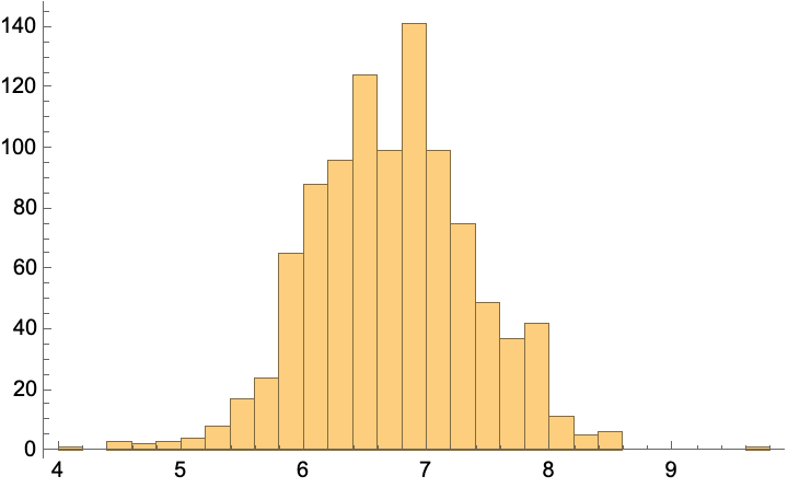
(*{-0.223916, -0.947164, 0.203167, -0.945561, -0.851039, 0.0911935, -1.10973, -0.761609, 0.668289, -0.341423, 0.31335} -> 6.*)

At least roughly, this looks like a better estimate than we had in the supervised approach. (Of course, this is just ML-by-vibes, and you should construct a more rigorous evaluation, but that exercise is left to the reader.)

ToJekyll["Semisupervised Twin Regression", "ml mathematica"]

Parerga and Paralipomena

, “loop”->Scaled[r]}` and eliminate the need to build in a summation function. This would also facilitate returning a history of each type of loss during the training cycle.

1. (27 Jan 2024) An alternative is to use the LossFunction option to set the hyperparameter scaling, in the form `LossFunction -> {“mse”->Scaled[1.-r] ↩