Comparing student success rates with the Beta distribution
[teaching dei mathematica statistics Sarah Maurer asks: The DEI community uses an disparity index (which is the ratio of outcomes of a a group of interest relative to the outcomes in the total population of students) as a way to measure disparate outcomes for students (for example, the DFW rate ). But this seems like it does not handle errors associated with small numbers of events. And what is a meaningful effect? Is there a better way to do this? The Beta-distribution to the rescue…
An example
Starfleet Academy has a population of Earthlings and Martians enrolled in Intro to Astronavigation. Eighty (80) of the 100 Earthlings enrolled pass the course. Similarly, 4 of the 5 Martians enrolled pass the course. The disparity index would suggest that this is an equitable outcome as the ratios are the same:
{80/100., 4/5.}

(*{0.8, 0.8}*)
disparityIndex[groupPass_, groupTotal_, allPass_, allTotal_] := (groupPass/groupTotal)/(allPass/allTotal)

disparityIndex[4, 5, 80 + 4, 100 + 5] // N

(*1.*)
But can we really say that Martians have equally good outcomes? If one borderline Martian fails, then it looks really bad!
disparityIndex[3, 5, 80 + 3, 100 + 5] // N

(*0.759036*)
And if a borderline Martian were to pass, it would seem as if the Martians had much better outcomes than the Earthlings!
disparityIndex[5, 5, 80 + 5, 100 + 5] // N

(*1.23529*)
There must be a better way.
Prelude: Modeling the outcomes as a sum of Bernoulli trials
What if we frame the problem in the following way: Suppose each group of students (Earthlings, Martians) is assigned a coin that results in passing the course with probability p, and flipping the coin determines their outcome in the course. The bias on the coin reflects all possible factors (prior preparation, socioeconomic, discrimination by the instructor, grit, inherent intellectual superiority, etc.). What is the distribution of coin weights, p, given an observed sample of outcomes?
Stated more formally, the observed class pass/fail outcomes are like a a coin that returns success with probability p (i.e., a Bernoulli trial). A round of n experiments corresponds to counting the number of successes in that series, i.e., a Binomial distribution. For a given observation of k successes, there are different p values that give rise to that outcome. As an illustrative example, we can ask what are the probabilities that a coin of p will give k=4 successes in n=5 trials. This is merely the probability density function:
binomialPDF[n_, k_] := PDF[BinomialDistribution[n, #], k]*(n + 1) &
Note that the PDF of the Binomial coefficient (normalised for n trials) has the following analytical form :
binomialPDF[n, k][p]

Note the need for a normalization constant (n+1):
Integrate[
  binomialPDF[5, 4][p],
  {p, 0, 1}]

(*1*)
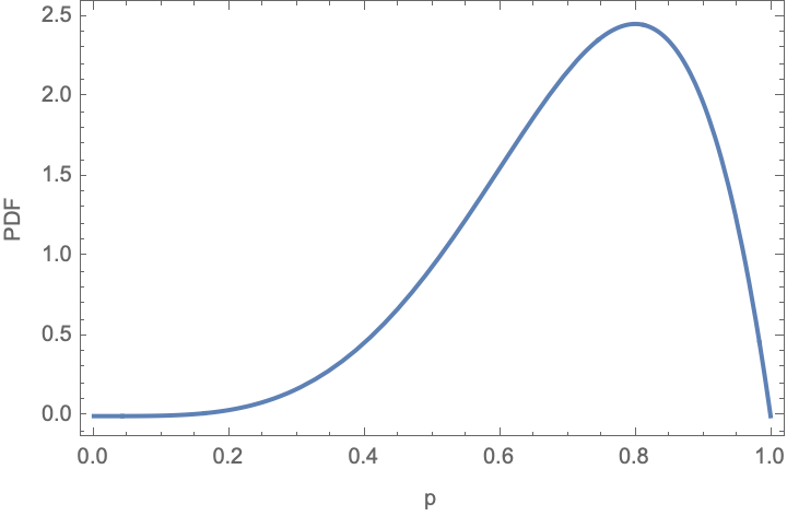
Returning to our example, what does the PDF look like for the n=5, k=4 example?
Plot[
  binomialPDF[5, 4][p] ,
  {p, 0, 1},
  Frame -> True, FrameLabel -> {"p", "PDF"}]

The maximum of this distribution corresponds to the simple average expectation from the trials:
FindMaximum[{
   binomialPDF[5, 4][p],
   0 < p < 1}, p]

(*{2.4576, {p -> 0.8}}*)
Note that while there can be a small chance of this outcome occurring, even if p is very small:
binomialPDF[5, 4][0.2]

(*0.0384*)
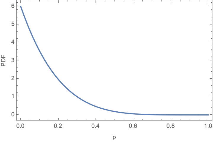
Note that this type of analysis is equally applicable to the case where we observe no successes at all (k=0):
Plot[
  binomialPDF[5, 0][p],
  {p, 0, 1}, PlotRange -> All,
  Frame -> True, FrameLabel -> {"p", "PDF"}]

The Beta Distribution
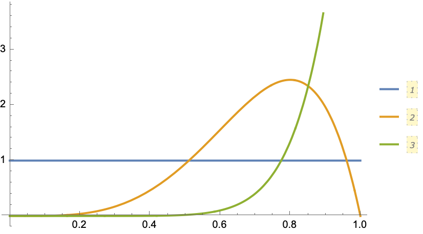
The function we derive above is actually well known in (Bayesian) statistics as the BetaDistribution. For example, Downing’s Think Bayes has a chapter on this problem. A few concrete cases to consider:
-
(blue)
BetaDistribution[1, 1]corresponds to a uniform prior at the start of the experiment with no trials–we have no information about the coin and therefore assume that any value of p between 0 and 1 is equally possible. -
(green)
BetaDistribution[10, 1]corresponds to observing 9 passes and zero failures. -
(orange)
BetaDistribution[5, 2](orBetaDistribution[1+4, 1+1]) corresponds to our Martians in the problem. That is, we add to the first index for each successful pass and add to the second index for each fail.
Plot[
  {PDF[BetaDistribution[1, 1], p],
   PDF[BetaDistribution[5, 2], p],
   PDF[BetaDistribution[10, 1], p]},
  {p, 0, 1},
  PlotLegends -> Automatic]

Treating the Martian/Earthling DEI Problem with the Beta Distribution
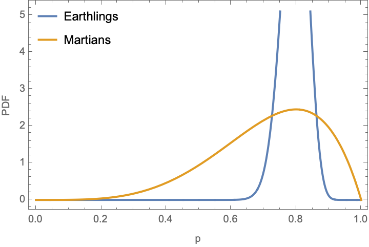
Begin by defining a convenience function for taking pass/fail numbers and converting them into distributions. Then we can plot the probability density functions of each distribution:
distribution[pass_Integer, fail_Integer] := BetaDistribution[1 + pass, 1 + fail]

earthlings = distribution[80, 20];
martians = distribution[4, 1];

Plot[
  {PDF[earthlings, p], PDF[martians, p]},
  {p, 0, 1},
  PlotLegends -> Placed[{"Earthlings", "Martians"}, {Left, Top}],
  Frame -> True, FrameLabel -> {"p", "PDF"}]

Although the maximum likelihood estimate for p is the same (i.e., the maxima of the distributions are centered at the same value), Martians are a worse bet than Earthlings:
Probability[m < e, {e \[Distributed] earthlings, m \[Distributed] martians}] // N

(*0.6413*)
(unless we convert this to a numerical result Mathematica will display a nice rational fraction, because at the end of the day it is just a counting problem that can be solved eactly)
This is really interesting and perhaps surprising. Although our disparity index calculation suggested they had the same outcome, Martians may be less likely to pass (on average) than Earthlings because of the uncertainty about their distribution from a fewer number of examples. That being said, this difference is far from any of the typical statistical significance level (should you believe in those things).
We can also determine the 90% confidence interval on p for each group based on these observations:
Quantile[earthlings, {0.05, 0.95}]

(*{0.72541, 0.856241}*)
Quantile[martians, {0.05, 0.95}]

(*{0.418197, 0.93715}*)
Clearly the distribution of Martian p are quite wide, and encompass the Earthling ones. Thus, it does not seem that there is clear evidence of any systematic advantage or disadvantage for Martian students at the Academy. Kirk out.
ToJekyll["Comparing student success rates with the Beta distribution", "teaching dei mathematica statistics"]