Three mathematical models for machine learning and high-throughput experimentation
[machine-learning probability Since the seminal 2018 Mexico City report, there has been increased interest in developing autonomous research systems–aka, self-driving laboratories–that combine machine learning (ML) with robotic experimentation. (For recent perspectives on this, see Stach et al. 2021 and Yano et al. 2022.). At least historically, automated experimentation implied high-throughput experimentation (HTE) with the goal of achieving large data scale. An alternative are continuous systems, where experiments are performed one at a time–these seem like they are optimal for incorporating learning into the process. How does HTE enable ML? Or vice versa? The goal is to get some intuitions that can be used to inform a provocative perspective article on ML for exceptional materials. It is also inspired by some ideas from a blog post on High-Variance Management (and corresponding Julia notebook), with examples from show business.. In this post, we explore a few simple mathematical models for this interplay and limits of ML and HTE…
Model 1: Binomial model
Premise: We assume that we have a machine that is capable of performing N experiments, and the probability of success for a single experiment (as guided by a ML model ) is p. With what probability is at least one success observed? (I am told models like this are used in venture capital—how many companies do I have to invest in to get at least one Google or Facebook?) You can work this out by hand in terms of the probability of not getting a winner for some choice of p and N, but I will just show off how easy it is to do this symbolically in Mathematica:
Probability[d > 0,
  {d \[Distributed] BinomialDistribution[n, p]},
  Assumptions -> (n > 0 && Element[n, Integers] && Element[p, PositiveReals])]

(*1 - (1 - p)^n*)
What does this look like as we modify p and N?
pSuccess[p_, n_] := 1. - (1 - p)^n

Plot[
  {pSuccess[0.001, n], pSuccess[0.01, n], pSuccess[0.10, n]},
  {n, 1, 200},
  PlotRange -> All,
  Frame -> True, FrameLabel -> {"Number of experiments, N", "p(Success)"},
  PlotLegends -> Placed[{"p = 0.1%", "p = 1%", "p = 10%"}, Top]]
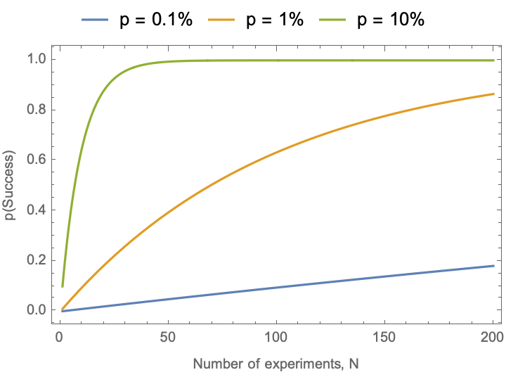
Conclusion: This is a pretty obvious conclusion. High-throughput experimentation increases N. Machine learning methods are intended to increase p. These have a synergistic effect, but their effect is essentially static. Furthermore, increasing p pays better rewards than increasing N.
Limits of the model: The models does not learn anything from the experiments–the success probability is the same. And all that matters is the total number of experiments that get performed in aggregate–there is no sense of batches. Active learning can improve the ML model by increasing dp/dt. Autonomous operation can improve both p and N by reducing the time delay to perform experiments using a model that improves p, and increasing dN/dt by automating the cycle. [Compound interest analogy: active learning in the loop is equivalent to compounding interest more frequently] The underlying assumption of this equation, of identical and independently distributed probabilities, does not describe the underlying distributions found in many materials science problems. This framework does not incorporate experimental or model uncertainties.
Model 2: Normal distribution step model
Premise: We assume that we have a machine that is capable of performing N experiments per batch. The machine is guided by a ML algorithm whose goal is to select a batch of experiments to try. The current state of knowledge of the model is described by x, which starts at x = 0. To make a discovery, we must reach a state of knowledge of x = 100. At each epoch, the algorithm selects new experiments that are a normal distribution around the best experimental result to date. (In other words, ML provides a store of knowledge, and has some sort of local, but imperfect awareness of improvement.) After each batch of experiments, the algorithm is retrained and generates new experiments around the best experimental result found to date. This gives us two free parameters: the batch size N and the standard deviation of the normal distribution predictions around the current best knowledge of the system–effectively how bold the model is in its extrapolations. We’ll assume that a baseline ML algorithm has a unit standard deviation, and that an appropriately designed ML algorithm for discovering exceptional materials may be able to increase this to a larger value.
How many steps are needed to reach the goal?
For concreteness, consider the case where we start from x=0 and ask how many iterations are required to reach an extreme material target x = 100. We will assess this by Monte Carlo:
Clear[iteration]
iteration[nSamples_Integer][start_ : 0, stdDev_ : 1] := With[
    {move = Max@RandomVariate[#, nSamples] &@NormalDistribution[start, stdDev]},
    Max[move, start] (*return whatever is largest*)]

continueQ[position_] := position < 100 (*stopping criterion*)

simulate[iterationFn_] := Length@NestWhileList[iterationFn, 0, continueQ];
simulate[iterationFn_, nIter_Integer] := ParallelTable[simulate[iterationFn], {nIter}]

Histogram[#, Automatic, "PDF", AxesLabel -> {"Epochs", "PDF"}] & /@ {
   simulate[iteration[1], 10^4], simulate[iteration[96], 10^4]}

Conclusion: As predicted, increasing the batch size from N = 1 (continuous iteration) to N=96 decreases the total number of batches required from ~250 to ~42. This suggests that if the N=96 batch can be performed in less than 250/42 (~6) times the amount of time that the N=1 batch can be performed, then we will find the solution in less elapsed time. However, it is worth noting that we had to consume 4296 = 4032 resources to do this, i.e . 16-times more resources as the *N = 1 continuous experiments. This might be relevant if experiments are more expensive than labor.
Quantifying the typical improvement size in a batch
Suppose we look at a single batch: How much improvement can be expected if we increase the batch size, given our normal distribution model? (Asymptotically, the limit of the maximum of a large number of samples from a normal distribution defines an ExtremeValueDistribution commonly referred to as a Gumbel distribution, but Gumbel discovered a few distributions, and Mathematica uses GumbelDistribution for the minimum value…) :
improvementPerBatch[batchSize_, stdDev_ : 1] := Around@Table[
     Max@RandomVariate[#, batchSize] &@NormalDistribution[0, stdDev],
     {10^4}]

improvementResult = ParallelTable[{2^n, improvementPerBatch[2^n]}, {n, 0, 16}];
ListLogLinearPlot[improvementResult,
  Frame -> True, FrameLabel -> {"Batch Size, N", "Improvement Per Batch"}]
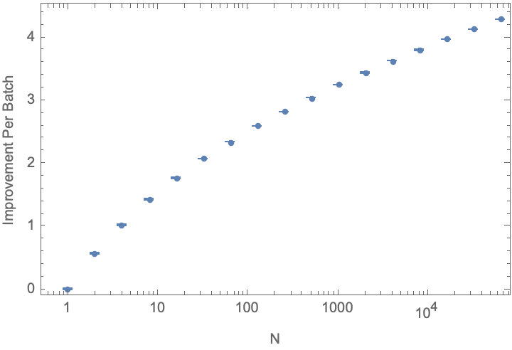
Conclusion: There are diminishing returns to increasing automation scale; improvements scale less than the logarithm of the batch size.
varianceImprovementResult = ParallelTable[{s, improvementPerBatch[96, s]}, {s, 1, 10}]
ListPlot[varianceImprovementResult, Frame -> True, FrameLabel -> {"Std. Dev", "Improvement Per Batch"}]

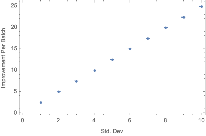
What does the tradeoff between the number of experiments in a batch and the standard deviation of the model look like? Show this as a contour plot:
result = ParallelTable[
    {Log[10, 2^n], s, improvementPerBatch[2^n, s]},
    {n, 16}, {s, 1, 10}];
ListContourPlot[
  Flatten[result, 1],
  FrameLabel -> {"\!\(\*SubscriptBox[\(Log\), \(10\)]\)(N)", "Std. Dev."}]
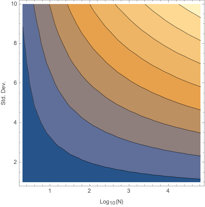
Conclusion: This model captures the idea that there is a synergy between high variance and high throughput–you unleash more power of having high throughout if you can simultaneously try riskier samples.
Limitations: While the state of knowledge improves over time, our ability to make improvements at each step remains constant. That is, our knowledge is cumulative, but does not have a compound-interest type effect.
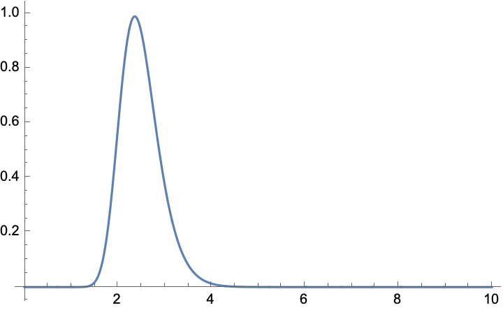
Addendum to Model 2: You can compute the PDF of the maximum value in a batch of N draws from a Gaussian distribution analytically. It’s fun to pencil it out in terms of error functions, but we can also just let the computer do the work:
f = PDF@OrderDistribution[{NormalDistribution[], n}, n]

For example, suppose a batch of 96; let’s plot the PDF of the maximum value in the batch, and estimate the maximum likelihood value
Plot[f[x] /. n -> 96, {x, 0, 10}, PlotRange -> All]
NMaximize[f[x] /. n -> 96, x]

(*{0.988625, {x -> 2.36023}}*)
Model 3: Probability of success is a function of current knowledge
Premise: Like the normal step model, we assume that we start at x = 0 and have to reach x = 100 to be successful. We assume that we have a machine that is capable of performing N experiments per batch. A ML algorithm has some value p of picking a winner, which starts very low. If one winner is found, we advance to x+1. The probability of success is given by p = (x+1)/100–i.e., we assume that at the early stages we know very little and as we amass better data we get better at picking the winner. This seems to make sense in the asymptotic limits: at x = 0 we know very little and at x = 99 we have a sure bet about the next step. You could always scale down the denominator if you thought a 1% initial chance of improvement was too optimistic (and indeed we will look at that later). But first some initial intuition by brute-force Monte Carlo:
step[x_, nTrials_, pScale_ : 100.] := With[
   {increment = Boole@GreaterThan[0]@Total@RandomVariate[#, nTrials] &@BernoulliDistribution[(x + 1)/pScale]},
   x + increment]
model3results = Table[simulate[step[#, 2^n] &, 10^4], {n, 0, 7}];
Around /@ model3results
ListPlot[%, Frame -> True, FrameLabel -> {"\!\(\*SubscriptBox[\(Log\), \(2\)]\) N", "Iterations"}]
Histogram[#, Automatic, "PDF"] & /@ model3results

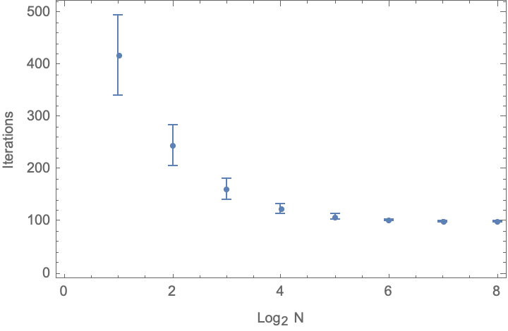

Conclusion: If you can run 128 experiments per batch, you always gets at least one success, so each iteration gets you to the next stage, and you more or less conclude in 100 iterations. But if you run only one experiment at a time, it typically takes 418 iterations to get to the success mark–slow progress at the beginning, and accelerating as we proceed. Interestingly, this is even more pessimistic than the second model that we examined–using these large batches we get a 4x acceleration, at the cost of a 128*100/418 = 30x increase in the number of experiments. And if each batch of 128 automated experiments takes more than 4x the time of running a single experiment, then we would get to the solution faster by just running the single experiments (even if they do fail a lot in the beginning).
What if we are more pessimistic and assume only a 0.01% chance of success in each round (increasing to only 1% in the end)? (I actually tried this by brute force but it was too slow–predicted times of over an hour, so I modified the code below to only compute a single version)
model4results = Table[simulate[step[#, 2^n, 10^4] &, 10^4], {n, {7}}];
(Warning: This takes a long time to compute if you are only running a single experiment because you run many epochs without success. See below for a smarter version of this than direct simulation.). Even with 128 experiments per batch, we need 382 epochs to reach the goal:
Around /@ model4results

Conclusions: This starts to capture some of the idea of cumulative learning during the process. HTE is most beneficial for the early stages–when know almost nothing and most experiments will fail. It becomes less essential as you learn more and progress to the next stage is easier. This suggests the most fruitful use of HTE may be to perform very high throughput and fast, but potentially noisy initial experiments and then to replace these with careful one-at-at-ime style experiments as the campaign proceeds.
Passing thoughts: This has some flavor similarity to gamblers ruin type problems. The relatively simple form of the probabilities of getting from one state to another may allow us to work out an analytical solution if we put our mind to it.
Making our simulation fast by modeling it as a discrete Markov process
You can treat this model as a DiscreteMarkovProcess, with a probability of getting to the next state which we derived in the binomial model above. The matrix will be mostly sparse with only on-diagonal and one-off-diagonal terms to get to the next state. Then just compute the mean time to reach the end with FirstPassageTimeDistribution. For easy of implementation, assume we start at state x = 1 and go to state x = 100 (as indexing is more naturally from 1 in Mathematica):
Clear[matr]
matr[nTrials_Integer, pScale_] :=
  SparseArray[
   { {100, 100} -> 1.,
    {i_, i_} -> (1. - (i /pScale))^nTrials,
    {i_, j_} /; (j == i + 1) -> (1 - (1. - (i /pScale))^nTrials)},
   {100, 100}]
mp = DiscreteMarkovProcess[1, matr[1, 100]];
data = RandomFunction[mp, {0, 800}] (*simulate the markov process as a sanity check*)
ListPlot[data]

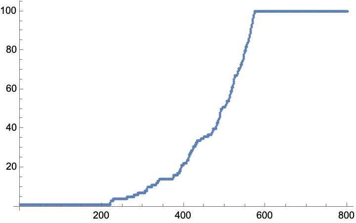
Now that we know it works, let’s compute the mean as a function of the batch size (in powers of two), plotting the result (on various log scales). We’ll consider a very pessimistic problem where our initial state of knowledge only gives us a 0.01% = (1/10^4) probability of making an initial advance, increasing only to a 1% chance of improvement in the last stages. In contrast to the brute-force Monte Carlo simulation above, this calculation now runs almost instantaneously:
results3 =
   Table[
    With[
     {mp = DiscreteMarkovProcess[1, matr[2^n, 10^4]]},
     {2^n, Mean@FirstPassageTimeDistribution[mp, {100}]}],
    {n, 0, 8}]

ListLogLinearPlot[%,
   Frame -> True, FrameLabel -> {"Batch size", "Epochs required"}]

ListLogLogPlot[%%,
  Frame -> True, FrameLabel -> {"Batch size", "Epochs required"}]

(*{ {1, 51773.8}, {2, 25911.7}, {4, 12980.7}, {8, 6515.36}, {16, 3282.93}, {32, 1667.21}, {64, 860.331}, {128, 458.823}, {256, 261.619}}*)
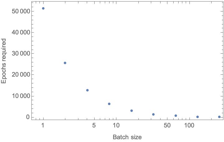
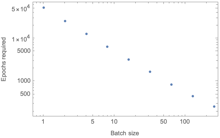
Conclusion: We require several order of magnitude more epochs to reach a result if we perform experiments one at a time–and reduce this to a few hundred epochs if we perform experiments en masse. In the end, the average cost is not much different–if we run 128 experiments in parallel we require only about 13% more resources (128*468/51773) would have been required if we run the experiments one at a time, and reduce the number of epochs required by a factor of 113. So like the examples above, the HTE machinery must be much faster than the serial, sequential experimentation (for example, time delays induced with characterization etc.) to realize the benefit in elapsed time.
ToJekyll["Three mathematical models for machine learning and high-throughput experimentation",
  "machine-learning, probability"]
Parerga and Paralipomena
- 03 Feb 2023: There are probably some nice analytical versions that one can devise using first-passage models in statistical physics. See First look and textbook by Sidney Redner. That is, define a diffusive process of some type (corresponding to the above), and find a closed solution in 1D
- (summer 2023): Some of the intuitions gleaned from this study made their way into a perspective article in JACS
- (03 Jun 2024) A fourth model might be to consider a “product-of-Gaussians” type scenario. For example there are different capabilities, each with a normal distribution, but to be successful one needs to combine them. This was discussed in terms of scientific productivity by Shockley (1957) and for general business perfomance by Boyle and Aguinus (2012). In this type of model, we might imagine that different types of synthesis and characterization capabilities are modeled as normal distributions; after Shockley, it would be easier for an 11-capability instrument to make a 10-capability discovery. Parallelism of courses helps buy more samplign opportunities, but can be outsmarted with better methodology.