Object-oriented programming in Mathematica

At its heart, Mathematica is a term replacement language, and includes primitives for both functional programming and procedural programming. But what about object oriented programming (OOP)? An interesting blog post by Hirokazu Kobayashi showed me how to get Mathematica down with OOP…

An Example

Let’s create some random numbers and divide into a 80/20% train-test split. We will want to develop an object which can store the observed minimum and maximum (MinMax) of the training set, and then apply that transformation (using Rescale) to any subsequent dataset. Let’s set up some example data

example = RandomVariate[NormalDistribution[], 1000];
{train, test} = ResourceFunction["TrainTestSplit"][example];

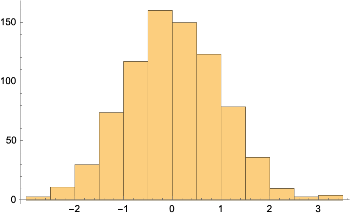
Histogram[train]
MinMax[train]
MinMax[test]

(*{-2.73525, 3.33049}*)

(*{-2.77628, 2.87314}*)

Instance-Preceded OOP

One strategy is so-called “instance proceeded OOP”. In this formation, the name of the instance leads our expression.

For the sake of showing the independence of our object, let us define fit and transform variables. We’ll later use these as the method names, and so the purpose of this is merely to show how the object orientation strategy avoids namespace conflicts.

{fit, transform} = {3, 5};

Now, let’s define our object:

Clear[MinMaxScalerInit, scaler, scaler2] 
 
MinMaxScalerInit[self_] := Module[
   {minMaxTrain = {0, 1}}, (*instance variables; set a default value*)
   
  (*set instance variables by memoization*) 
   self[fit[x_List]] := minMaxTrain = MinMax[x]; 
   
  (*use instance variables as you wish*) 
   self[transform[x_List]] := Rescale[x, minMaxTrain]; 
  ]

Here’s how to apply it:

MinMaxScalerInit[scaler] (*initialize the object, creating an instance `scaler` *)
scaler@fit[train] (*use scaler's fit method *)
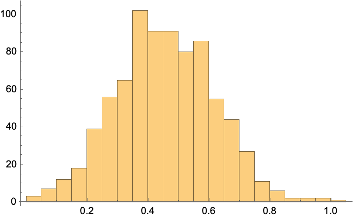
Histogram[  
  scaler@transform[train] ] (*use the scaler's transform method*)


(*{-2.73525, 3.33049}*)

Once fit has been obtained and stored in scaler, it can be applied to any other function:

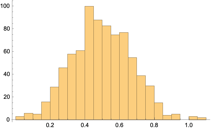
Histogram[
  scaler@transform[test], 
  PlotRange -> { {0, 1}, Automatic}]

Multiple scaler objects can be created. Let’s create another one just to see how it behaves independently

MinMaxScalerInit[scaler2]
scaler2@fit[test]
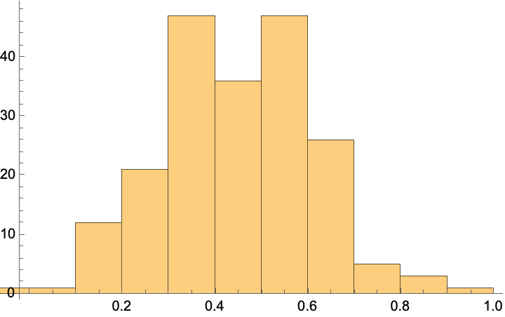
Histogram[scaler2@transform[train]]


(*{-2.77628, 2.87314}*)

You can always add a dedicated initialization (init) method for the purpose of setting initial variables.

The instance-preceded style is similar to python, where the OOP pattern is instance.method().

Method-Preceded OOP

An alternative approach is Method-Proceeded OOP; in this case we will take advantage of our ability to set UpValues of the expressions. This has the advantage of appearing slightly more idiomatic in Mathematica, as the methods look like functions that we apply to the object that is created. The difference is that they are specific to the object instances that we create, rather than being general patterns that can be applied to any input. Here we go:

Clear[MinMaxScalerInit, scaler] 
 
MinMaxScalerInit[self_] := Module[
    {minMaxTrain = {0, 1}}, (*define instance variables*)
    
   (*use UpValues to set definition of instance variables*) 
    fit[self[x_List]] ^:= minMaxTrain = MinMax[x]; 
    
   (*use UpValues to apply result*) 
    transform[self[x_List]] ^:= Rescale[x, minMaxTrain]; 
   ] 
  
 (*demo*)
MinMaxScalerInit[scaler]
fit@scaler[train] 
 
Histogram[
  transform@scaler[test], 
  PlotRange -> { {0, 1}, Automatic}]

(*{-2.73525, 3.33049}*)

Comment:

In neither of these patterns is it automatic to be able to retrieve instance variables; you need to define explicit getter methods.

##

• Flavors of OOP paradigms and their Mathematica implementation

ToJekyll["Object-oriented programming in Mathematica", "mathematica, programming, oop"]