Linear discriminant analysis

Bob LeSuer (aka BobTheChemist) asked: *“Because it’s Friday and I don’t want to grade, I’m doing multivariate analysis with #Mathematica (yes, grading ranks that low). PCA is working nicely. @JoshuaSchrier do you have strategies for doing LDA with cross-validation?” This set me off on a Saturday morning project to learn Linear Discriminant Analysis (not the local density approximation, although you can read about implementing that in my book). The best article I found was Sebastian Raschka’s “Linear Discriminant Analysis–Bit by Bit” which describes the basic idea, and then explains the LDA process in 5-steps, using the Fisher Iris dataset and an implementation in python. (Gabriel Peyre has a nice animation, though.) LDA is similar to Principle Components Analysis (PCA), in that the goal is to project a dataset onto a lower-dimensional space, but with an additional goal of finding axes that maximize the separation between different classes of outcomes. After reducing your data in this way, you can then use your favorite machine classifier method. Let’s see how to implement LDA in Mathematica…

Intuition

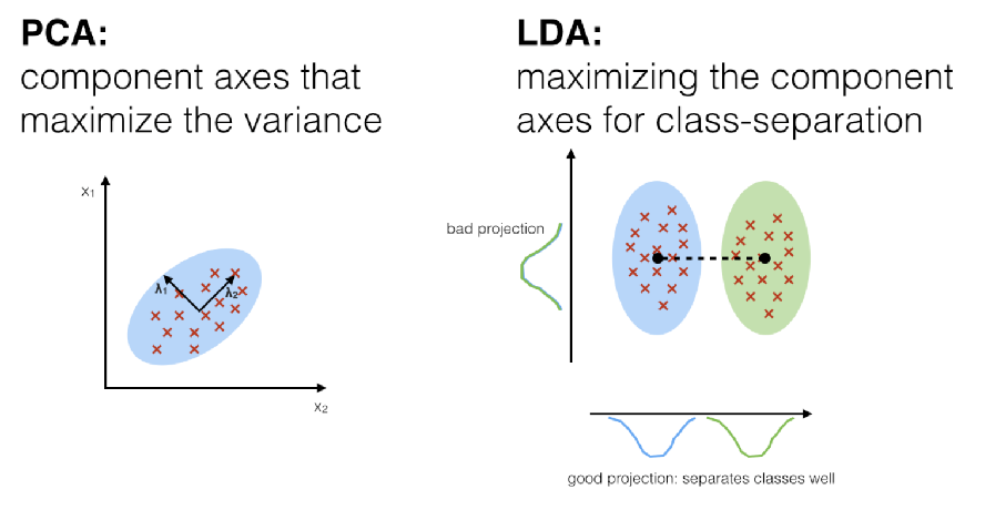
Our goal is to reduce the dimensions of a d -dimensional dataset by projecting it onto a k-dimensional subspace (where k<d). To do this, we compute eigenvectors (the components) using the data set and collect them in a so-called scatter-matrices (i.e., the in-between-class scatter matrix and within-class scatter matrix). The corresponding eigenvalues tell us about the magnitude of each eigenvector. If some eigenvectors are much larger than others, we might only keep those with the highest eigenvalues, since they contain more information about our data. Eigenvalues close to zero contain very little information, and can be removed. TWe will keep the k largest eigenvalues, as they contain the most information; if they are comparable to each other, then that suggests that the data is already in a “good” feature space and cannot be reduced further. This is quite similar to PCA–the main difference is that we are now tracking between and within-class scatter and incorporating that information into our selection of the top k components.

0lelj0tqkgnk2

Image source: https://sebastianraschka.com/Articles/2014_python_lda.html#a-comparison-of-pca-and-lda

Step-by-Step Implementation

This closely follows Raschka’s article, so I won’t repeat his text (which is quite lucid).

Get the data

Let’s use the classic Fischer Iris dataset: I’m wrapping these in “Short” to just show a preview of what a typical Mathematica machine learning data looks like (values -> output list), and how we group these by class (dropping the class label):

Short[
   data = ExampleData[{"MachineLearning", "FisherIris"}, "Data"]] 
 
Short[
  groupedByClass = Map[First, #, {2}] &@GroupBy[Last]@data]

0l909m5ciqpk4

0ctbyve2jg62q

Step 1: Computing the d-dimensional mean vectors

We can compute the mean of each class by mapping the Mean operator over it; we do not actually need this variable, as we’ll do it on-the-fly below

meanVectors = Mean /@ groupedByClass

(*<|"setosa" -> {5.006, 3.428, 1.462, 0.246}, "versicolor" -> {5.936, 2.77, 4.26, 1.326}, "virginica" -> {6.588, 2.974, 5.552, 2.026}|>*)

Step 2: Computing the Scatter Matrices

2.1 Within-class scatter matrix $S_w$

Si[data_] := (Length[data] - 1)*Covariance[data]
withinClassScatterMatrix[allData_] := Total[Si /@ allData] 
  
 (*apply to our problem*)
MatrixForm[
  Sw = withinClassScatterMatrix[groupedByClass]]

1mm8s70xi706e

(Wrapping MatrixForm around the assignment so the output looks pretty.)

2.2 Between-class scatter matrix $S_B$

betweenClassScatterMatrix[allData_] := With[
   {meanVectors = Mean /@ allData, 
    overallMean = Mean[Join @@ Values@allData], 
    n = Length /@ allData}, 
   Total@MapThread[
     #1*KroneckerProduct[ (#2 - overallMean), (#2 - overallMean)] &, 
     {Values[n], Values[meanVectors]}]]

(*apply to our problem*)
  MatrixForm[
   Sb = betweenClassScatterMatrix[groupedByClass]]

044v511qs06c9

Step 3: Solving the generalized eigenvalue problem for the matrix

Comment: The global phase (sign) can vary depending on the eigensolver; in this case the signs below are opposite those in the reference tutorial; this is a quirk of the particular eigenvalue solver package that is used, but has no great significance. What we care about is the magnitude:

{eigVals, eigVecs} = Eigensystem[Inverse[Sw] . Sb]

(*{ {32.1919, 0.285391, -4.98501*10^-15, 1.12983*10^-15}, { {0.208742, 0.386204, -0.554012, -0.70735}, {-0.00653196, -0.586611, 0.252562, -0.769453}, {-0.416713, 0.434054, 0.485412, -0.634289}, {0.834292, -0.386936, -0.389037, 0.0537322}}}*)

Take a look at the first eigenvalue …

eigVals[[1]]

(*32.1919*)

and its corresponding eigenvector:

eigVecs[[1]]

(*{0.208742, 0.386204, -0.554012, -0.70735}*)

Take a look at each of the eigenvectors:

eigVals

(*{32.1919, 0.285391, -4.98501*10^-15, 1.12983*10^-15}*)

Step 4: Selecting linear discriminants for the new feature subspace

4.1. Sorting the eigenvectors by decreasing eigenvalues

Comment: Sorting the eigenvectors is unnecessary, as eigenvalues are returned in descending order of magnitude. But we can still look at the amount of explained variance

varianceExplained = eigVals/Total[eigVals]

(*{0.991213, 0.0087874, -1.53492*10^-16, 3.47882*10^-17}*)

The way to read this: The first eigenvector captures 99.1% of the variance, the second captures and additional 0.8%, the remainder are essentially zero:

4.2. Choosing k eigenvectors with the largest eigenvalues

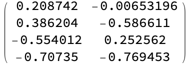
Form a transformation matrix W from the top eigenvectors that we will use to transform the data. (Again; this is the same to within a global phase (sign) of the results in the reading)

MatrixForm[
  W = Transpose@eigVecs[[1 ;; 2]]]

1tljub97jx5ca

Step 5: Transforming the samples onto the new subspace

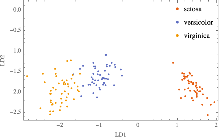
Xlda = (# . W) & /@ groupedByClass; (*apply W to each class*) 
 
ListPlot[Xlda, 
  PlotTheme -> "Scientific", 
  FrameLabel -> {"LD1", "LD2"}, 
  FrameLabel -> "LDA:Iris projection onto the first 2 linear discriminants", 
  PlotLegends -> Placed[Automatic, {Right, Top}]]

01bzys5y3q56q

Comment: As the signs of the first eigenvector are flipped, this reverses the right-left symmetry compared to the Raschka’s result, but the conclusion is the same.

Putting this together into a cross-validated classifier

We’ve built up the process above to illustrate the reasoning. Now let’s just put the code in one place and define a convenience wrapper so that it can be used as a drop-in dimensionality reduction tool

(*helper functions defined above*)
   Si[data_] := (Length[data] - 1)*Covariance[data] 
   
   withinClassScatterMatrix[allData_] := Total[Si /@ allData] 
   
   betweenClassScatterMatrix[allData_] := With[
     {meanVectors = Mean /@ allData, 
      overallMean = Mean[Join @@ Values@allData], 
      n = Length /@ allData}, 
     Total@MapThread[
       #1*KroneckerProduct[ (#2 - overallMean), (#2 - overallMean)] &,
       {Values[n], Values[meanVectors]}]] 
   
  (*return the total variance and W transformation matrix for a data set, selecting a target dimension*)
   LDADetermine[data_, targetDimensions_Integer : 2] := Module[
    (*define local variables*) 
     {groupedByClass, Sw, Sb, eigVecs, eigVals, totalVarianceExplained, howMany}, 
     
    (*perform calculation*) 
     groupedByClass = Map[First, #, {2}] &@GroupBy[Last]@data; 
     Sw = withinClassScatterMatrix[groupedByClass]; 
     Sb = betweenClassScatterMatrix[groupedByClass]; 
     {eigVals, eigVecs} = Eigensystem[Inverse[Sw] . Sb]; 
     totalVarianceExplained = Accumulate[ eigVals/Total[eigVals]]; 
     
    (*return...*) 
     {totalVarianceExplained[[targetDimensions]], (* total variance*)
      Transpose@eigVecs[[1 ;; targetDimensions]] (* W*)} 
    ] 
   
  (*define a way for applying the transform to arbitrary datasets*) 
   LDAApply[W_][x_ -> y_] := Chop[(x . W)] -> y (*apply to one data item.  Chop out tiny imaginary components*)
   LDAApply[W_][data_List] := LDAApply[W] /@ data (*apply over a set of data items*)

Demo:

Perform LDA on the Fisher Iris example data using our convenience wrapper

data = ExampleData[{"MachineLearning", "FisherIris"}, "Data"];
{varianceExplained, W} = LDADetermine[data, 2]

(*{1., { {0.208742, -0.00653196}, {0.386204, -0.586611}, {-0.554012, 0.252562}, {-0.70735, -0.769453}}}*)

Apply the function to our data and build a classifier:

Classify[
  LDAApply[W][data], 
  Method -> {"NearestNeighbors", "NeighborsNumber" -> 3}]

039arp2mds0j4

Cross validation (the hard way)

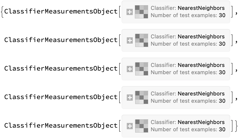
We can probably get away with a 1-nearest neighbor classifier, so let’s try it. The function below performs a single random 80/20% train/test split on the input data, then constructs a classifier model (using the Methods specified by the second argument after generating a LDA transform of a specified number of dimensions. It returns a ClassifierMeasurementObject that describes the performance on the test set.

oneFold[data_, 
   classifierMethod_ : {"NearestNeighbors", "NeighborsNumber" -> 1}, targetDimension_Integer : 2] := 
  Module[{train, test, captured, W, classifier}, (*local variables*)
   {train, test} = ResourceFunction["TrainTestSplit"][data]; 
   {captured, W} = LDADetermine[train, targetDimension]; 
   classifier = Classify[LDAApply[W][train], Method -> classifierMethod]; 
   ClassifierMeasurements[classifier, LDAApply[W][test]] 
  ]

Apply this to perform a 5-fold cross validation:

results = Table[oneFold[data], {5}]

1mh5sw3148wng

Determine Mean and Standard deviation of each of these test measurements

Around[#["Accuracy"] & /@ results]

0gu2cpf4tp7n3

Many other prediction characterization properties are available:

results[[1]]["Properties"]

(*{"Accuracy", "AccuracyBaseline", "AccuracyRejectionPlot", "AreaUnderROCCurve", "BatchEvaluationTime", "BestClassifiedExamples", "ClassifierFunction", "ClassMeanCrossEntropy", "ClassRejectionRate", "CohenKappa", "ConfusionDistribution", "ConfusionFunction", "ConfusionMatrix", "ConfusionMatrixPlot", "CorrectlyClassifiedExamples", "DecisionUtilities", "Error", "EvaluationTime", "Examples", "F1Score", "FalseDiscoveryRate", "FalseNegativeExamples", "FalseNegativeNumber", "FalseNegativeRate", "FalsePositiveExamples", "FalsePositiveNumber", "FalsePositiveRate", "GeometricMeanProbability", "IndeterminateExamples", "LeastCertainExamples", "Likelihood", "LogLikelihood", "MatthewsCorrelationCoefficient", "MeanCrossEntropy", "MeanDecisionUtility", "MisclassifiedExamples", "MostCertainExamples", "NegativePredictiveValue", "Perplexity", "Precision", "Probabilities", "ProbabilityHistogram", "Properties", "Recall", "RejectionRate", "Report", "ROCCurve", "ScottPi", "Specificity", "TopConfusions", "TrueNegativeExamples", "TrueNegativeNumber", "TruePositiveExamples", "TruePositiveNumber", "WorstClassifiedExamples"}*)

#[{"MCC"}] & /@ results

(*{ {<|"setosa" -> 1., "versicolor" -> 1., "virginica" -> 1.|>}, {<|"setosa" -> 1., "versicolor" -> 0.906327, "virginica" -> 0.931891|>}, {<|"setosa" -> 1., "versicolor" -> 1., "virginica" -> 1.|>}, {<|"setosa" -> 1., "versicolor" -> 1., "virginica" -> 1.|>}, {<|"setosa" -> 1., "versicolor" -> 1., "virginica" -> 1.|>}}*)

NotebookFileName[]
ToJekyll["Linear discriminant analysis", "ML statistics chemometrics"]

(*"../journals/science/2021.04.02_linear_discriminant_analysis.nb"*)