Parrondo and Portfolio Diversification

Michael Stutzer, a professor of finance at University of Colorado, Boulder has written about how portfolio diversification can be thought of as a Parrondo-like problem. Essentially, one can think about rebalancing a portfolio to include some assets that have negative expected real returns (for example, treasury bonds) as being analogous to the Parrondo paradox, and he constructs a simple binomial model to explain this in a pedagogically simple way. The results will not be surprising to any Boglehead…

For sake of argument, we will consider a hypothetical stock with a 6% expected real return and volatility of 40%, and a hypothetical risk-free asset (let’s call it a treasury bond) with a negative real return of -1%. We’ll consider a 30 year period, with annual compounding.

drift = 0.06;
volatility = 0.40;

Full Geometric Brownian Motion Simulation

First, let’s examine the behavior of a single asset, modeled by geometric brownian motion:

gbmSimulation = RandomFunction[
    GeometricBrownianMotionProcess[drift, volatility, 1], 
    {1, 30, 1}, 10^5] 
 
gbmResult = gbmSimulation["LastValues"];

Let’s analyze the outcomes. We also want to estimate the probability that we lose money:

fractionLost[trials_] := N@Mean@Boole@Map[LessThan[1]]@trials

Here are the results:

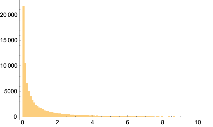
Histogram[gbmResult, {0.1}]
#[gbmResult] & /@ {Mean, Median, fractionLost}

(*{6.31947, 0.551884, 0.60764}*)

While the mean (expected value) is positive (predicting that we should have $6.23 for every starting $1), this is only because of the long tail of wins. The median case is that we lose money (we have only $0.55 for each starting $1), and 60% of the time we have lost money.

Defining an Equivalent Binomial Model

To simplify the discussion, Stutzer introduces an equivalent binomial lattice model, wherein at each discrete time we flip a fair coin: if heads we multiply our current wealth by (1+u) and if tails we multiply it by (1-d). We can find the appropriate values of u and d by fitting to the expected return (1+drift) and volatility in our example):

Solve[
  (1 + u)/2 + (1 - d)/2 == (1 + drift) && (*expected return*)
   Sqrt[((1 + u)^2 + (1 - d)^2)/2 - (1 + drift)^2] == volatility, (*volatility*)
  {u, d}, PositiveReals]

(*{ {u -> 0.46, d -> 0.34}}*)

Using these fitted parameters, we can simulate the outcome. I’ll just hand write a function for this:

trial[u_, d_, n_ : 30] := Times @@ RandomChoice[{(1 + u), (1 - d)}, n] 
 
binomialResult = Table[trial[0.46, 0.34], {10^5}];
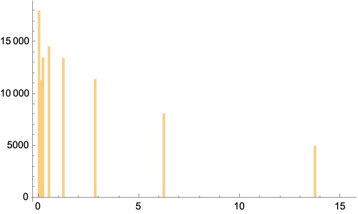
Histogram[binomialResult, {0.1}]
#[binomialResult] & /@ {Mean, Median, fractionLost}

(*{5.52688, 0.573392, 0.57237}*)

The results are qualitatively the same as for the geometric Brownian motion case: Positive expected value (dominated by rare “big win” scenarios), median loss, and most players lose. However, because of the discrete changes, we only get clumps of results, rather than the continuum of outcomes in GBM.

The Value of Diversification

Suppose that we have two stocks that are uncorrelated but have the same drift and volatility as above. We can imagine rebalancing the portfolio each year to keep an equal amount. How does this change the results after 30 years?

twoAssets[u_, d_][t_] := {t/2, t/2} . RandomChoice[{(1 + u), (1 - d)}, 2] 
 
rebalanceTrial[stepFn_, initial_ : 1, n_ : 30] := Nest[stepFn, initial, n] 
 
twoAssetResults = Table[
    rebalanceTrial[twoAssets[0.46, 0.34]], 
    {10^5}];
#[%] & /@ {Mean, Median, fractionLost}

(*{5.77629, 1.95962, 0.33927}*)

Notice how the expectation value has decreased, but the median is now “winning” as opposed to losing…and we end up in the red only 30% of the time. This should not be surprising–each of our choices has a long-tail of wins, and so we are essentially buying more chances at having that win. As an exercise for the reader, imagine that you diversify across the total stock market…

FinancialData["VTSAX", "Name"]

(*"Vanguard Total Stock Market Index Fund Admiral Shares"*)

Parrondo-like Diversification Game

The Parrondo-like variation is to consider diversifying between the stock (which has has a positive expectation, but negative median return) and a hypothetical risk-free asset with negative expectation (i.e., guaranteed to lose some amount every year). Stutzer considers the latter to have a real return of -0.1%, but it is even more dramatic to consider that it has a real return of -1%, as I shall do below. The relationship with Parrondo is that it seems apparently paradoxical that including an asset with guaranteed loss should improve our performance (compared to our original single-asset investment). But what do the simulations say? As before, we’ll rebalance into a 50-50 portfolio each year and simulate this with the binomial lattice model:

assetPlusRiskFree[u_, d_, riskFreeReturn_][t_] := {t/2, t/2} . {RandomChoice[{(1 + u), (1 - d)}], 1 + riskFreeReturn} 
 
assetPlusRiskfreeResult = Table[
     rebalanceTrial[assetPlusRiskFree[0.46, 0.34, -0.01]], 
     {10^5}]; 
 
#[%] & /@ {Mean, Median, fractionLost}

(*{2.07847, 1.17179, 0.43025}*)

Obviously, we can’t win as much (so the mean goes down), but the median investor sees a positive return, and the fewer investors who have lost money over time. Thus, “paradoxically” including a losing asset helps, acting like a ratchet that prevents us from losing too much money in any one trial, analogous to the ratchet-version of the Parrondo paradox.

NotebookFileName[]
ToJekyll["Parrondo and Portfolio Diversification", "finance investing parrondo montecarlo"]

(*"/Users/jschrier/Dropbox/journals/mathematica/2022.08.06_parrondo_diversification.nb"*)