Maximum entropy coin toss, revisited

Suppose that you roll a die many times and learn that the average value is 5–what is the most likely (maximum entropy) distribution of the probabilities? Last week we solved this by brute force…today we’ll solve it by considering the Gibbs Distribution (aka Boltzmann’s Law)…

probabilities = Table[ Exp[-beta *i ], {i, 6}]/Sum[Exp[-beta*j], {j, 6}];
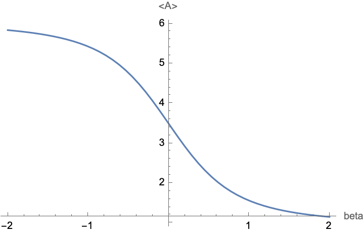
expectationValue = Range[6] . probabilities;
Plot[expectationValue, {beta, -2, 2}, AxesLabel -> {"beta", "<A>"}]

Now solve the expression for beta, and use the result to determine the probabilities:

soln = Solve[expectationValue == 5, beta, Reals]
probabilities /. soln // N

(*{ {0.0205324, 0.0385354, 0.0723234, 0.135737, 0.254752, 0.47812} }*)

Which agrees with our previous brute force optimization. The advantage is that we are only optimizing over a single variable, rather than 6 dimensions as before.

If you’re old-school, you can do this by hand by replacing lambda = Exp[-beta], and express each of the probabilities as lambda^i. Substitute these probabilities into the expectation value and then solve this polynomial equation for lambda.

Pro-tip: You can get a higher paying job if you say softmax instead of Gibbs Distribution :-)

ResourceFunction["ToJekyll"]["Maximum entropy coin toss, revisited", "probability optimization thermodynamics"]