Kelly Optimal Betting With Discrete Data
[gambling optimization kelly I was intrigued by an article on John Parkhill’s blog about the discrete version of the Kelly Criterion. The core idea is that one uses a series of samples of returns and then determines a Kelly-optimal strategy for those samples; the advantage of working with discrete samples (rather than “probabilities” deduced from such data) is that it captures realistic correlations. The Kelly optimal bet vector, $c_k$, (i.e., the fraction of your wealth to wager on each asset k) is found by minimizing the following loss function…

where S is the total number of samples, and i is an index over samples, and $r_{\text{ik}}$ is the observed return of asset k at time i. John’s blog does some implementations in PyTorch and then introduces a partially-baked nontransitive die example (but only demonstrates things with a single roll). My goal here was to think through this a bit (especially as I enjoyed reading William Poundstone’s book Fortune’s Formula on Kelly, Shannon, and friends), and make a very simple implementation, and build out application to the non-transitive dice example.
A simple example: Rolling Simple Dice and Nontransitive Dice
Suppose we have a set of dice, defined below. These have the interesting property of being non-transitive. We begin by defining the die and a small function that rolls them some number of trials:
die1 = {2, 2, 4, 4, 9, 9};
die2 = {1, 1, 6, 6, 8, 8};
die3 = {3, 3, 5, 5, 7, 7};
dice = {die1, die2, die3};

roll[die_List, number_Integer : 10^5] := RandomChoice[die, number]
Next, define a function to test how often one die wins compared to another, given a list of samples:
percentWins[rolls1_List, rolls2_List] := N@Mean@Boole@MapThread[Greater, {rolls1, rolls2}]

Table[
  With[
   {rollsI = roll@dice[[i]],
    rollsJ = roll@dice[[j]]},
   If[i != j,
    {i, j, percentWins[rollsI, rollsJ]},
    Nothing]
  ],
  {i, 3}, {j, 3}]

(*{ { {1, 2, 0.55506}, {1, 3, 0.4432}}, { {2, 1, 0.44764}, {2, 3, 0.55562}}, { {3, 1, 0.55571}, {3, 2, 0.44621}}}*)
It is also fun to define a payoff function on each die, which returns about 1% on average):
payoff[face_] := (face/10) - 0.49
SetAttributes[payoff, Listable]
This is an interesting choice as it makes the mean payoff is about 1% for each die individually:
MeanAround@payoff@roll[#] & /@ dice

What’s the best bet?
The premise of the Kelly Criterion is that you do not want to bet too small (as this does not maximize gain), or too big (which can cause you to lose all your money). Let’s define some functions that define the payout, and then a wrapper function that takes those bets. I will define two versions of this, one that takes a scalar bet (single process) and one that takes a vector bet:
bet[percentBet_?NumericQ][total_, payoff_] := total + total*percentBet*payoff
bet[percentBet_List][total_, payoff_] := total + total*percentBet . payoff

bet[percentBet_, sampleOutcomes_] := FoldList[ bet[percentBet], 1, sampleOutcomes]
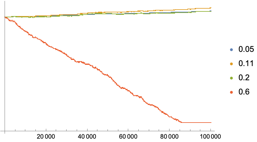
Let’s see how this performs on a log plot….
With[
   {sampleOutcomes = payoff@roll@die1},
   ListLogPlot[
    {bet[0.05, sampleOutcomes],
     bet[0.11, sampleOutcomes], (*this is  Kelly-optimal bet for this system*)
     bet[0.20, sampleOutcomes],
     bet[0.6, sampleOutcomes]},
    PlotLegends -> {0.05, 0.11, 0.20, 0.6}]] // Quiet

As we can see, the Kelly optimal bet gives a higher return, and avoids the crashing that we see with strategy 4.
Now implement the Kelly Loss
So how do we find the Kelly-optimal bet size, $c_k$? We want to minimize the loss function:

For a scalar case, this is pretty simple (we take advantage of the fact that addition by a scalar and Log are both Listable functions, so they apply to each term in the input list:
kellyLoss[cAssets_?NumericQ, rAssets_List] :=
  -Mean[
    Log[(1 + cAssets*rAssets)]]
It is not much more difficulty when this is a vector –we just take a dot-product for each of the samples, implementing the sum in a straightforward, pythonic way.
kellyLoss[cAssets_?VectorQ, rAssets_?MatrixQ] :=
  -Mean[
    Table[
     Log[(1 + cAssets . rik)], {rik, rAssets}]]
This of course is bound to be less efficient, even if it is somewhat easier to understand or implement. So let’s play a little code golf to make it more idiomatic. We can replace the Table construction with a Map, or better yet…just treat this as a matrix-vector multiply, taking advantage of the listable addition and Log functions:
(*code golf: version 2*)
kellyLoss2[cAssets_?VectorQ, rAssets_?MatrixQ] := -Mean[Log[(1 + cAssets . #)] & /@ rAssets]

(*code golf: version 3*)
kellyLoss3[cAssets_?VectorQ, rAssets_?MatrixQ] := -Mean@Log[(1 + rAssets . cAssets)]
These all give identical results (second outcome in the list), but it’s an order of magnitude faster to use the third strategy. (We could get even more speedups if we use NumericArray instead of the general purpose lists, but its irrelevant for us here)
example2 = payoff[roll[#]] & /@ {die1, die2, die3} // Transpose;
kellyLoss[{0.1, 0.1, 0.4}, example2] // RepeatedTiming
kellyLoss2[{0.1, 0.1, 0.4}, example2] // RepeatedTiming
kellyLoss3[{0.1, 0.1, 0.4}, example2] // RepeatedTiming

(*{0.179052, -0.00274043}*)

(*{0.027883, -0.00274043}*)

(*{0.0219753, -0.00274043}*)
To close this section, let’s just define these functions for the single and multiple cases:
Clear[kellyLoss]
kellyLoss[cAssets_?NumericQ, rAssets_List] := -Mean[Log[(1 + cAssets*rAssets)]]
kellyLoss[cAssets_?VectorQ, rAssets_?MatrixQ] := -Mean@Log[(1 + rAssets . cAssets)]
Minimizing the Kelly Loss for a single asset
I suppose you can do something fancy like a neural net (treat $c_k$ as a trainable set of weights), but any minimizer will do. Let’s start with a single asset to try to evaluate:
example = payoff@roll@die1; (*example data:  returns on die 1*)

Plot[
  kellyLoss[c, example],
  {c, 0, 1}]

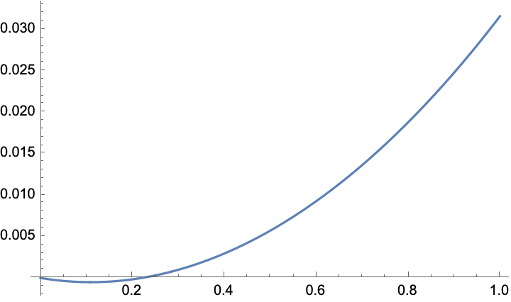
So there’s a clear unique minimum, just as we expected! Now let’s find it
Minimize[
  {kellyLoss[c, example],
   c > 0}, (*make sure the bet is constrained*)
  c]

(*{-0.000508904, {c -> 0.10971}}*)
As stated earlier, the optimal bet is around 11% for this system.
Pricing multiple assets
Now let’s define a more complicated system–we have all three of the die. These are uncorrelated, but the distribution of payouts varies. Although the average payout for each die is 1%, the payouts are distributed differently.
payoff /@ {die1, die2, die3}
Mean /@ %

(*{ {-0.29, -0.29, -0.09, -0.09, 0.41, 0.41}, {-0.39, -0.39, 0.11, 0.11, 0.31, 0.31}, {-0.19, -0.19, 0.01, 0.01, 0.21, 0.21}}*)

(*{0.01, 0.01, 0.01}*)
Let’s generate some sample returns (for each bet), and use this to Minimize. It’s pretty straightforward, taking advantage of the VectorGreaterEqual symbol (which looks much nicer when not rendered in markdown) to constrain these to be positive reals…
example2 = payoff[roll[#]] & /@ {die1, die2, die3} // Transpose;
Minimize[
  {kellyLoss[c, example2],
   c \[VectorGreaterEqual] 0},
  c \[Element] Vectors[3, Reals]
 ]

(*{-0.00280708, {c -> {0.103281, 0.101441, 0.37662}}}*)
(As an aside, we can also add additional constraints about the betting. We might have to enforce a “don’t bet more than the whole bankroll” rule in some cases (it turns out not to matter here):
Minimize[
  {kellyLoss[c, example2],
   c \[VectorGreaterEqual] 0,
   Total[c] <= 1},
  c \[Element] Vectors[3, Reals]]

(*{-0.00280708, {c -> {0.103281, 0.101441, 0.37662}}}*)
Alternatively, we could also force ourselves that we must bet everything on each round by introducing an equality (this is unlikely to do well…sometimes it is better not to bet):
Minimize[
  {kellyLoss[c, example2],
   c \[VectorGreaterEqual] 0,
   Total[c] == 1},
  c \[Element] Vectors[3, Reals]]

(*{-0.00132387, {c -> {0.185132, 0.176845, 0.638024}}}*)
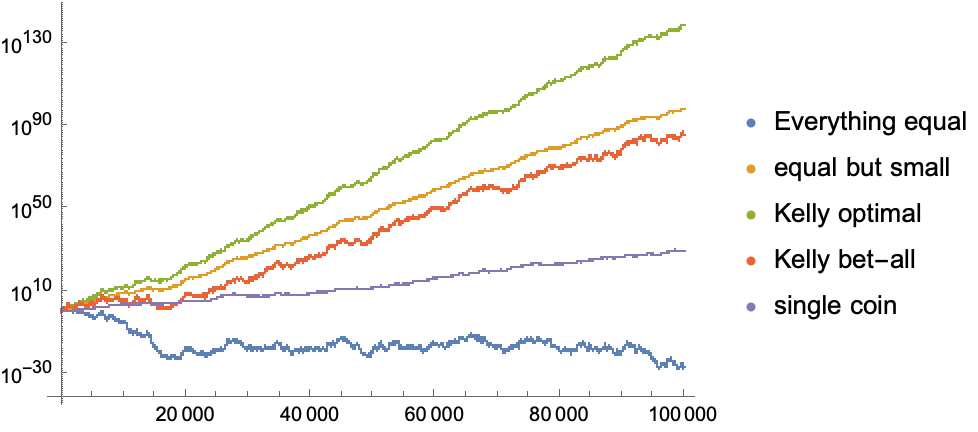
How well these different strategies perform on a newly generated test set (just to avoid the appearance of overfitting…)?
example3 = payoff[roll[#]] & /@ {die1, die2, die3} // Transpose;

ListLogPlot[
  {bet[{0.33, 0.33, 0.33}, example3],(*everything equal*)
   bet[{0.11, 0.11, 0.11}, example3],(*everything equal...but small*)
   bet[{0.12, 0.13, 0.37}, example3],(*Kelly optimal*)
   bet[{0.20, 0.20, 0.60}, example3],(*bet everything each round*)
   bet[{0.11, 0, 0}, example3] (*just bet on coin 1*)
  },
  PlotLegends -> {"Everything equal", "equal but small", "Kelly optimal", "Kelly bet-all", "single coin"}
 ]

What’s amazing here is that the returns are better with the three dice than the best you can achieve with a single die, even though each of them returns 1% on average.
Fun with asset allocation
Let’s try to model how to build a Boglehead 3-fund style portfolio (total stock market, total international stock market, total bond market), using daily return as the bet outcome:
lastYear =
   FinancialData[#, "Return", {"Jan. 1, 2020", "Dec. 31, 2020"}]["Values"] & /@ {"VTSAX", "VTIAX", "VBTLX"} // Transpose;
Total /@ Transpose[lastYear]

With[
  {r = Chop@Normal@lastYear}, (*QuantityMagnitude returns the numeric value of the percent, but we want it to return the fraction; we can do this with Normal*)
  Minimize[
   {kellyLoss[c, r],
    c \[VectorGreaterEqual] 0,
    Total[c] <= 1},
   c \[Element] Vectors[3, Reals]]]

(*{-0.000656705, {c -> {0.999978, 2.46692*10^-6, 5.07313*10^-6}}}*)
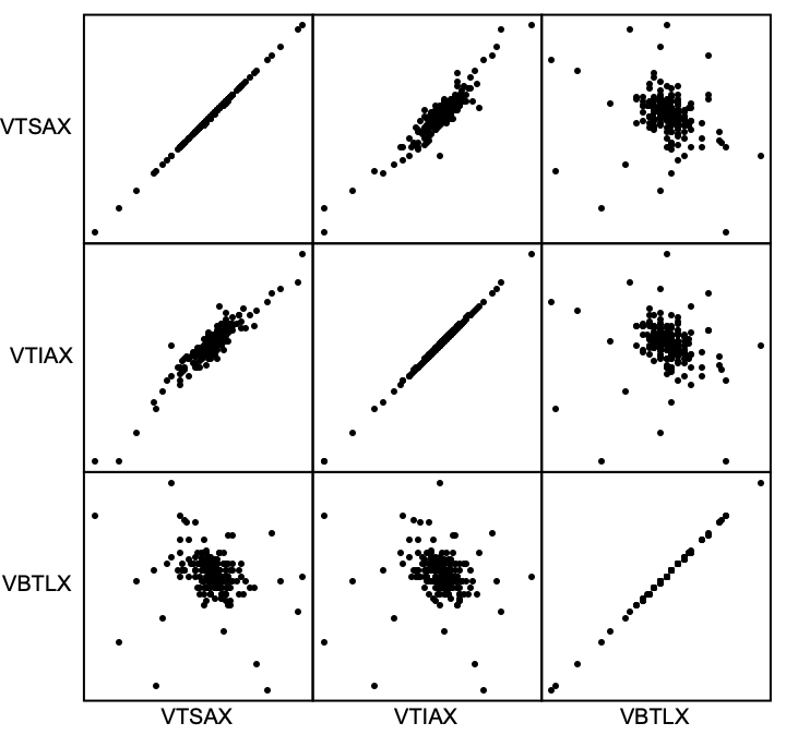
Interesting….the Kelly Bet says bet it all on Domestic Stocks; screw the bonds and international :-)
Note that this is not so weird. During this time period, US and international stocks were correlated, and stocks were anticorrelated with bonds, as one would expect…but the returns on bonds sucked over this time window.
ResourceFunction["PairwiseScatterPlot"][Normal[lastYear],
  "DataLabels" -> {"VTSAX", "VTIAX", "VBTLX"}]

NotebookFileName@EvaluationNotebook[]
ToJekyll["Kelly Optimal Betting With Discrete Data", "gambling optimization"];

(*"/Users/jschrier/Dropbox/journals/science/2021.08.27_johnparkhill.nb"*)