Bezier the Bookie
[probability gambling convexity Two gamblers go to a bookie to make a bet: Each pays a $1 to play a game in which they flip two coins. If both are tails, then player A wins, and receives $1.9 (his net return is +$0.9). If both are heads, then player B wins the $1.9. In the case of one head and one tail, there’s no clear winner, so both are out $1. How do the payoffs behave as a function as the probability of the coin goes from p(Heads) = 0 to 1? This straightforward probability problem has a nice (and perhaps unexpected) interpretation in terms of Bézier curves, which are more familiar in the context of computer graphics…
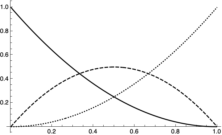
Bézier curves have a probabilistic interpretation–they are expressed in terms of the Bernstein basis is the probability of getting n heads when flipping a coin d times, where the probability of getting heads is x).
?BernsteinBasis

BernsteinBasis[d,n,x] equals $\left(
\begin{array}{c}
d
n
\end{array}
\right) x^n (1-x)^{d-n}$ between $0$ and $1$ and zero elsewhere.
Plot[
  {BernsteinBasis[2, 0, x],
   BernsteinBasis[2, 1, x],
   BernsteinBasis[2, 2, x]},
  {x, 0, 1}]
The expectation value is just the Bezier curve as a function of the probability, where the control points of the Bezier curve are the different payout scenarios:
pts = { {-1, 0.9}, {-1, -1}, {0.9, -1} };
Graphics[ {Blue, BezierCurve[pts], Red, Point[pts]}, ImageSize -> Small]
BezierFunction[pts][0.5]
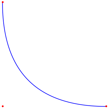
(*{-0.525, -0.525}*)
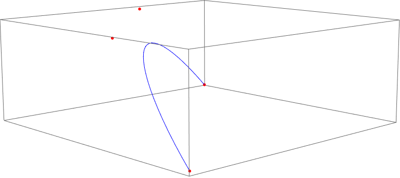
We can consider the Bookie’s return as a third dimension for our Bezier interpolation. Again, each control point in our Bezier curve defines the payouts from the perspective of each player (gambler 1, gambler 2, bookie):
pts = { {-1, 0.9, 0.1}, {-1, -1, 2}, {0.9, -1, 0.1} };
Graphics3D[ {Blue, BezierCurve[pts], Red, Point[pts]}]
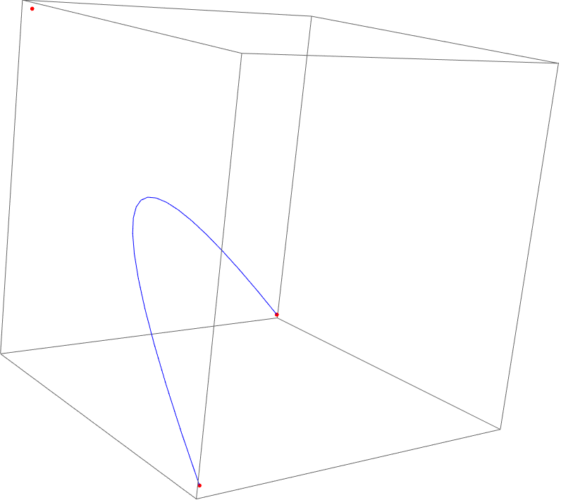
The bookie maximizes his reward when the coin is fair (p = 0.5):
BezierFunction[pts][0.5]

(*{-0.525, -0.525, 1.05}*)
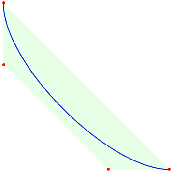
What if they extend the game to three coin tosses, and the bookie gives a consolation prize–getting two coin tosses gives a payout of +$1.2 to the "best-two" winner. The Bernstein basis is convex, so the expectation value (blue line) has to lie within the convex hull of the different outcomes (the different payout points)
pts = { {-1, 0.9}, {-1, 0.2}, {0.2, -1}, {0.9, -1} };
Graphics[ {Blue, BezierCurve[pts], Red, Point[pts], Opacity[0.1], Green, ConvexHullMesh[pts]}, ImageSize -> Small]
pts = { {-1, 0.9, 0.1}, {-1, 0.2, 0.8}, {0.2, -1, 0.8}, {0.9, -1, 0.1} };
Graphics3D[ {Blue, BezierCurve[pts], Red, Point[pts], Opacity[0.1], Green}]
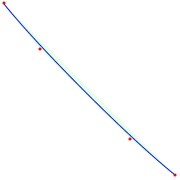
The problem becomes less interesting as the bookie becomes less greedy:
pts = { {-1, 0.9}, {-0.6, 0.4}, {0.4, -0.6}, {0.9, -1} };
Graphics[ {Blue, BezierCurve[pts], Red, Point[pts], Opacity[0.1], Green, ConvexHullMesh[pts]}, ImageSize -> Small]
NotebookFileName@EvaluationNotebook[]
ToJekyll["Bezier the Bookie", "probability gambling convexity"];

(*"/Users/jschrier/Dropbox/journals/mathematica/2021.11.13_bezier_the_bookie.nb"*)