Parrondo's Paradox

Parrondo’s Paradox (discovered in 1996) is a curious scenario in which by alternating between two losing (negative expected value) games a player can win (achieve positive expected value). Paul Nahin in Digital Dice describes the following variant: Consider games in which flipping heads results in winning $1, and tails results in losing $1. Game A has you flip a biased coin that returns heads with probability 1/2-epsilon. Clearly this is a losing game (negative expected value) for epsilon >0. Game B has you flip a coin that depends on your current wealth, M. If M is divisible by 3 then you flip a coin that shows heads with probability 1/10-epsilon; otherwise you flip a coin that shows heads with probability 3/4-epsilon. This too is a losing game (negative expected value). The “paradox” is that by alternating between these games, you can achieve a positive expected value over time…

Implementation

Comment: Mathematica has built in functions for manipulating random processes, but we do not use them here. We’ll consider epsilon = 0.005 as an example.

Clear[payoffForCoinFlip, gameA, gameB, alternate] 
 
payoffForCoinFlip[headsProbability_ : 1/2] := RandomChoice[{headsProbability, 1 - headsProbability} -> {+1, -1}] 
 
gameA[M_, epsilon_ : 0.005] := M + payoffForCoinFlip[1/2 - epsilon] 
 
gameB[M_, epsilon_ : 0.005] := M + If[Divisible[M, 3], payoffForCoinFlip[1/10 - epsilon], payoffForCoinFlip[3/4 - epsilon]] 
  
 (*alternate between games*)
alternate[M_, epsilon_ : 0.005] := RandomChoice[{gameA[M, epsilon], gameB[M, epsilon]}]

Results

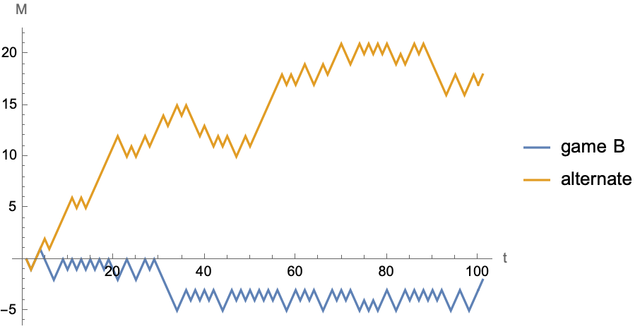
Plot a single trajectory

ListLinePlot[
  {NestList[gameB[#] &, 0, 100], 
   NestList[alternate[#] &, 0, 100]}, 
  PlotLegends -> {"game B", "alternate"}, 
  AxesLabel -> {"t", "M"}]

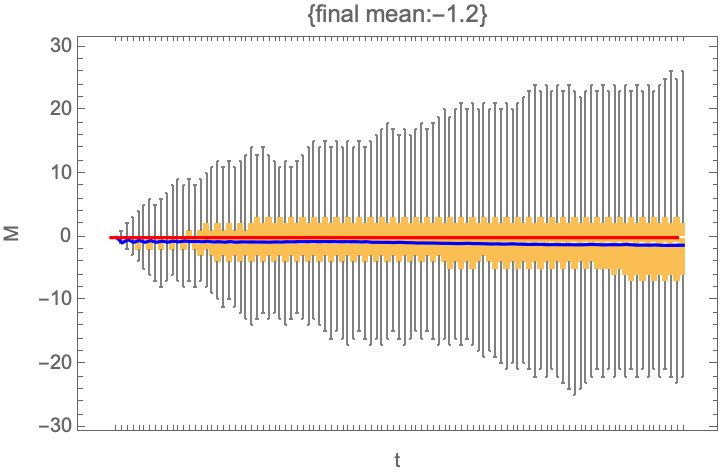
Ensemble averaging and visualization

Clear[trajectory, ensemble, visualize] 
 
trajectory[game_, M_, nFlips_ : 100, epsilon_ : 0.005][] := NestList[game[#, epsilon] &, M, nFlips] 
 
ensemble[trajectoryFn_, nTrials_ : 10^3] := Table[trajectoryFn[], {nTrials}] 
 
visualize[ensembleData_?MatrixQ, initialM_ : 0, nFlips_ : 100] := With[
   {groupedByTime = Transpose@ensembleData}, 
   With[
    {meanWithTime = Mean /@ groupedByTime}, 
    Show[
     BoxWhiskerChart[groupedByTime, FrameLabel -> {"t", "M"}, 
      PlotLabel -> {"final mean:" <> ToString@N@Last@meanWithTime}], 
     ListLinePlot[meanWithTime, PlotStyle -> Blue], 
     Plot[initialM, {x, 0, nFlips}, PlotStyle -> {Red}]]]]

visualize@ensemble@trajectory[gameB, 0]

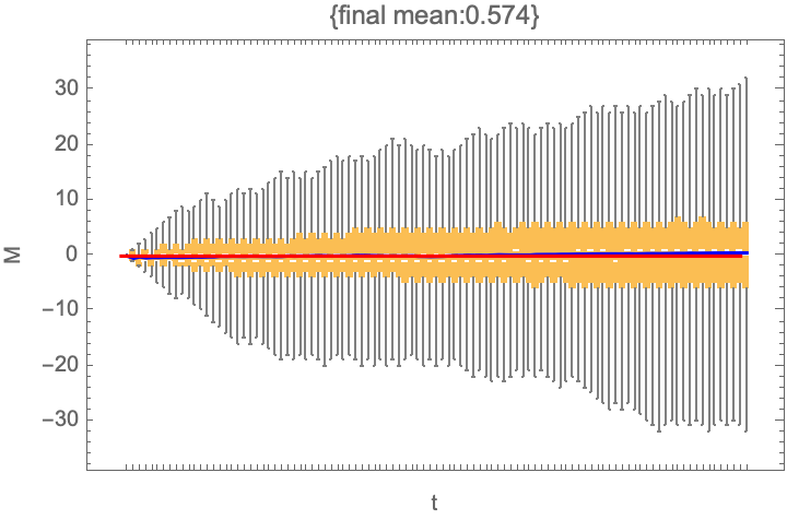
visualize@ensemble@trajectory[alternate, 0]

Further reading: Review article by Dinas & Parrondo discussing the problem in terms of Brownian ratchets. Also discusses modifications of the game to “social” settings and modification that don’t depend on knowing the total capital amount, but instead use history of wins and losses. [https://arxiv.org/abs/1410.0485]

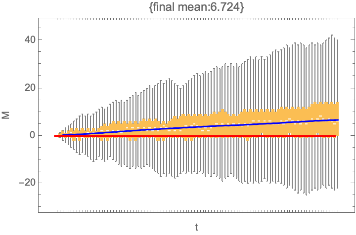
Bonus: What is the optimal Parrondo game sequence?

Answer: ABABB [https://arxiv.org/abs/1409.6497]

Implementation strategy: Overload the trajectory[] function so that it can take a list of games.

trajectory[gameSequence_List, M_, nFlips_ : 100][] := With[
   {fullSequence = Take[#, nFlips] &@Flatten@Table[gameSequence, {Ceiling[nFlips/Length[gameSequence]]}]}, 
   ComposeList[fullSequence, M]]

visualize@ensemble@trajectory[{gameA, gameB, gameA, gameB, gameB}, 0]

Comment: Non-default values of epsilon can be provided by using a list of pure anonymous functions, e.g.,

trajectory[{gameA[#, 0.005] &, gameB[#, .005] &, gameA[#, 0.005] &}, 0][] // Short

ToJekyll["Parrondo's Paradox", "gambling stochasticprocesses nahin montecarlo parrondo"]