Knuth's Toilet Paper Problem

One of my innocent pleasures is reading probability puzzle books, a habit I started with Paul Nahin’s Digital Dice. Chapter 8 in Nahin’s book presents Donald Knuth’s toilet paper problem (American Mathematical Monthly1984). Knuth’s paper begins as follows: “The toilet paper dispensers in a certain building are designed to hold two rolls of tissues, and a person can use either roll. There are two kinds of people who use the rest rooms in the building: big-choosers and little-choosers. A big-chooser always takes a piece of toilet paper from the roll that is currently larger, and a little-chooser always does the opposite. However, when the two rolls are the same size, or only one roll is nonempty, everybody chooses the nearest nonempty roll. When both rolls are empty, everybody has a problem. Let us assume that people enter the toilet stalls independently at random, with probability p that they are big choosers … If the janitor supplies a particular stall with two fresh rolls of toilet paper, both of length n, let Mn(p) be the number of portions left on one roll when the other roll first empties.” This problem can be solved by introducing a recurrence relationship, with some fun use of memoization for efficiency…

Initial Implementation

Some consideration of the problem leads us to write the following recurrence relationships:

Clear[KnuthM] 
 
KnuthM[n_, 0, p_] := n
KnuthM[n_, n_, p_] := KnuthM[n, n - 1, p]
KnuthM[m_, n_, p_] /; m > n > 0 := p*KnuthM[m - 1, n, p] + (1 - p)*KnuthM[m, n - 1, p] 
  
 (*define the single input wrapper form*)
KnuthM[n_, p_] := KnuthM[n, n, p]

Initial Application

Reproduce the analytic proof in the chapter

KnuthM[3, p] (*by default returns the full expression*)
% // Expand (*take previous result and expand into polynomial terms*)

(*p (2 (1 - p) + p) + (1 - p) (3 (1 - p) + p (2 (1 - p) + p))*)

(*3 - 2 p - p^2 + p^3*)

A first attempt to plot of $M_{200}(p)$

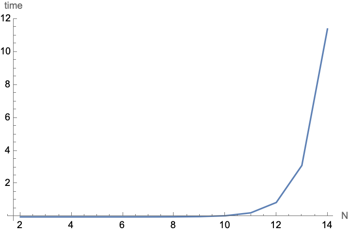
It is tempting to use this recursive result directly; however the number of terms expands tremendously as N increases. So this strategy is not going to work. Consider the Timing to evaluate the first few terms (shown below) as a warning…

({#, First@Timing@KnuthM[#, 0.5]}) & /@ Range[2, 14]

(*{ {2, 0.000041}, {3, 0.000024}, {4, 0.000061}, {5, 0.000178}, {6, 0.000563}, {7, 0.001849}, {8, 0.006331}, {9, 0.021513}, {10, 0.070539}, {11, 0.247147}, {12, 0.875677}, {13, 3.12324}, {14, 11.4004}}*)

ListLinePlot[%, AxesLabel -> {"N", "time"}, PlotRange -> All]

Performance boost with memoization

The alternative is to utilize memoization to “remember” intermediate results; this increases the amount of memory used, but saves the computational cost of recomputing the many values before. This is the functional version of the “matrix of values” described in Nahin’ s solution.

Implementation

Clear[KnuthM]
KnuthM[n_, 0, p_] := KnuthM[n, 0, p] = n
KnuthM[n_, n_, p_] := KnuthM[n, n, p] = KnuthM[n, n - 1, p]
KnuthM[m_, n_, p_] /; m > n > 0 := KnuthM[m, n, p] = p*KnuthM[m - 1, n, p] + (1 - p)*KnuthM[m, n - 1, p] 
  
 (*define the single input wrapper form*)
KnuthM[n_, p_] := KnuthM[n, n, p]

({#, First@Timing@KnuthM[#, 0.5]}) & /@ Range[2, 14]

(*{ {2, 0.000048}, {3, 0.000025}, {4, 0.000035}, {5, 0.00006}, {6, 0.00004}, {7, 0.000046}, {8, 0.00005}, {9, 0.000055}, {10, 0.000062}, {11, 0.00007}, {12, 0.000094}, {13, 0.000086}, {14, 0.00009}}*)

Comment: Observe the dramatic reduction of time, especially for the largest cases. A similar approach can be used for accelerating a symbolic expression, but this becomes unwieldy and slow for the very high order polynomial that gets produced. So instead, we’ll just utilize a numerical solution

Timing@KnuthM[200, 0.5]

(*{0.165553, 15.9477}*)

Notice that we’ve now memorized the result, so subsequent calculations are faster:

Timing@KnuthM[200, 0.5]

(*{0.000025, 15.9477}*)

Results

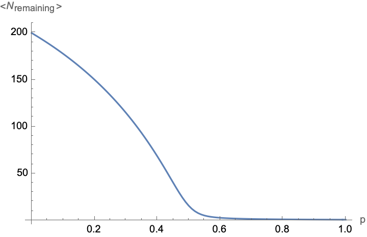
This ends up taking a trivial time to compute; use of ParallelTable takes advantage of multiple processors and also compiles the underlying functions, further accelerating the calculation

(results = ParallelTable[{p, KnuthM[200, p]}, {p, 0, 1, 0.01}];) // Timing 

(*{0.981225, Null}*)

ListLinePlot[results, AxesLabel -> {"p", "<\!\(\*SubscriptBox[\(N\), \(remaining\)]\)>"}]

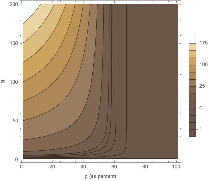
A fun application is that we’ve memoized all these results and can plot the behavior as both p and the initial N (using a problem-appropriate color theme):

results2 = ParallelTable[KnuthM[N, p], {N, 0, 200}, {p, 0, 1, 0.01}];

ListContourPlot[results2, 
  ColorFunction -> "CoffeeTones", PlotLegends -> Automatic, FrameLabel -> {"p (as percent)", "N"}, Contours -> {175, 150, 125, 100, 75, 50, 25, 10, 5, 4, 3, 2, 1}]

Excerpted from: 2019.06.10_DigitalDice.nb

ToJekyll["Knuth's Toilet Paper Problem", "recurrence probability"]